Performance Analysis of the Amplify-and-Forward Scheme under Interference Constraint and Physical Layer Security

http://dx.doi.org/10.7236/JIIBC.2014.14.1.179

JIIBC 2014-1-24

물리 계층 보안과 간섭 제약 환경에서 증폭 후 전송 기법의 성능 분석

Performance Analysis of the Amplify-and-Forward Scheme under Interference Constraint and Physical Layer Security

팜옥손, 공형윤

^*

Pham Ngoc Son, Hyung-Yun Kong

^*

요 약 언더레이 프로토콜은

2

차 시스템이나 인지된 사용자가

1

차 사용자의 품질 저하 없이 동일한 주파수를 사용 하는 인지 기술이다

.

또한

,

무선 환경의 중계 특성으로 인해

,

몇몇 노드는 도청 노드라고 불리며

,

다른 통신 링크를 위한 정보를 수신한다

.

이러한 이유로

,

물리 계층의 보안은 도청의 발생을 막기 위해 보안 성취율을 고려하여 응용된 다

.

본 논문에서는

,

물리 계층 보안과 간섭 제약 환경에서 증폭 후 전송 기법의 성능을 협력 통신 노드를 이용하여 분석한다

.

이 모델에서

,

중계기는 송신단에서 수신단으로의 신호 전송을 돕기 위해 증폭 후 전송 기법을 사용한다

.

우 수한 중계기는 기회주의적 중계기 선택 기법으로 선정되며

,

단 대 단 보안 성취율을 기초로 한다

.

시스템 성능은 보 안 성취율의 정전 확률로 평가된다

.

정전 확률의 상향

,

하향 한계는 국제 통계 채널 상태 정보

(CSI)

에 기초하며

,

또한

,

닫힌계로 유도한다

.

시뮬레이션 결과는 인지 네트워크는

1

차 사용자로부터 충분히 멀 때

,

중계기에서 도청 노드까지 의 거리가 중계기에서 수신단까지의 거리보다 큰 경우 시스템 성능이 향상된 것을 보여준다

.

Abstract The underlay protocol is a cognitive radio method in which secondary or cognitive users use the same frequency without affecting the quality of service (QoS) for the primary users. In addition, because of the broadcast characteristics of the wireless environment, some nodes, which are called eavesdropper nodes, want to illegally receive information that is intended for other communication links. Hence, Physical Layer Security is applied considering the achievable secrecy rate (ASR) to prevent this from happening. In this paper, a performance analysis of the amplify-and-forward scheme under an interference constraint and Physical Layer Security is investigated in the cooperative communication mode. In this model, the relays use an amplify- and-forward method to help transmit signals from a source to a destination. The best relay is chosen using an opportunistic relay selection method, which is based on the end-to-end ASR. The system performance is evaluated in terms of the outage probability of the ASR. The lower and upper bounds of this probability, based on the global statistical channel state information (CSI), are derived in closed form. Our simulation results show that the system performance improves when the distances from the relays to the eavesdropper are larger than the distances from the relays to the destination, and the cognitive network is far enough from the primary user.

Key Words : Cognitive radio, Interference constraint, Physical layer security, Underlay protocol, Cooperative communication, Amplify-and-forward, Opportunistic relay selection.

*정회원, 울산대학교 전기전자정보시스템공학부

접수일자 : 2013년 11월 14일, 수정완료 : 2014년 1월 15일 게재확정일자 : 2014년 2월 7일

Received: 14 November, 2013 / Revised: 15 January, 2014 / Accepted: 7 February, 2014

*Corresponding Author: [email protected]

School of Electrical Engineering, University of Ulsan, Korea

Ⅰ. Introduction

Cognitive radio is a protocol for effectively using spectrum in which a secondary or cognitive network cooperates with a primary network

^[1-2]

. In cognitive radio, the underlay protocol is a sharing method in which the secondary users use the same frequency as the primary users when transmitting their signals without affecting the quality of service (QoS) of the primary network. Hence, the secondary users must control their power so that the interference power of the primary user is less than a threshold value, which is called the interference constraint

^[1-2]

. In addition, because of the problems of wireless communication, including fading and obstacles, cooperative communication is an effective solution for enhancing system performance

^[3]

. In this model, the decode-and-forward, amplify-and-forward, and coded cooperation methods are used by relay nodes to help the source forward signals to the destinations. Methods to select the best relay have been proposed in many papers, such as partial relay selection

^[4-5]

and opportunistic relay selection

^[5]

through two hops during two timeslots. The partial relay selection method chooses the best relay based on the best quality at either the source-relay or the relay-destination, while the opportunistic relay selection method considers the highest end-to-end signal quality.

In a wireless communication environment, because of the broadcast characteristics of the signals, some nodes, called eavesdroppers nodes, try to obtain these signals illegally. Hence, Physical Layer Security is proposed to prevent illegal actions without using keys between the source and destination

^[6-7]

by using an achievable secrecy rate (ASR), which is a secret signal rate from the source to its desired destination. The methods to maximize this rate have been applied

^[6]

to enhance communication system performance. In system analysis problems with Physical Layer Security, all of the instantaneous channel state information (CSI) is known at every node (called global CSI), but in

practice, the statistical CSI of the source-primary user and relays-primary user links are available based on the long-term statistics of these nodes

^[7]

.

In this paper, we propose and analyze the system performance of the amplify-and-forward scheme under an interference constraint and Physical Layer Security, in which the best relay is chosen by the opportunistic relay selection method. The system performance is evaluated based on the outage probability of ASR. Our simulation results show that the system performance improves when the locations of the eavesdropper node are farther from the relays than the destination, and the cognitive network is farther from the primary network.

In addition, the exact expressions for the lower and upper bounds of the outage probability are provided, and we show that the cooperative communication model improves and outperforms direct transmission when number of relays is increased.

This paper is organized as follows: Section 2 describes the system; Section 3 calculates and analyzes the cognitive system performance using the outage probability of ASR; Section 4 presents the simulation results; and Section 5 summarizes our conclusions.

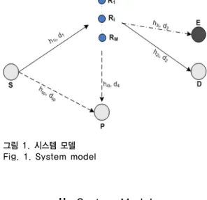
그림 1. 시스템 모델 Fig. 1. System model

Ⅱ. System Model

Fig. 1 presents the system model of the

amplify-and-forward scheme under an interference

constraint and Physical Layer Security. In Fig. 1, the secondary network includes a source S, a destination D, an eavesdropper node E, and relays Ri,

{ ^{1, 2,...,} }

i ∈ M , where S wants to transmit signals to the destination D with the help of M relays under an interference constraint at the primary network (node P) and Physical Layer Security against the eavesdropper node E. In this communication model, the source S and relays Ri will decrease their power so that the interference at the primary user P is below a threshold value, and the eavesdropper node E wants the signals of the S-D communication link without the agreement of S and D. We assume the following:

∙Each node has a single antenna.

∙Eavesdropper node E keeps a close watch on and is near the destination D.

∙All channels are flat and block Rayleigh fading channels in which the channel coefficients are constant in a packet interval and change from packet to packet.

∙The global channel state information (CSI) is available regarding any two nodes.

∙The additive white Gaussian noise (AWGN) at all relays and receiver nodes has the same zero mean and variance 

_

.

In Fig. 1,

(

h d

sp

^,

sp)

_, ( ^{h d}

_1i

^,

_1i

) _, ( ^{h d}

_2i

^,

_2i

) _, ( h d

3_i

,

3_i

) , and ( h d

4_i

,

4_i

) denote the Rayleigh fading channel coefficients and the link distances of S-P , S-Ri, Ri-D , Ri-E, and Ri-P, where i ∈ { 1,2,..., M } .

Set

2

sp

h

sp

ω = _, ω

_1i

= h

_1i²

_, ω

_2i

= h

_2i²

_, ω

_3i

= h

_3i²

and

2 4i

h

4i

ω = _{, which are} exponential random

variables with parameters λ

^sp

= ^d

^spβ

, λ

¹ⁱ

= d

^1β

= , λ

¹

2i

d

2^β 2

λ = = λ , λ

³ⁱ

= d

^3β

= λ

³

, and λ

⁴ⁱ

= d

^4β

= , λ

⁴

respectively, where β is a path-loss exponent.

In this paper, we propose an amplify-and-forward scheme under an Interference Constraint and Physical

Layer Security (called the AFICPLS protocol), where the best relay is chosen using an opportunistic relay selection (ORS) method. We assume that there is not a direct link from S to D or from S to E. The operation principle of this protocol is based on a time-division channel model, and is split into two time slots. In the first time slot, the source S broadcasts the signal ps to all secondary relays Ri. The signal received at the ith relay Ri, ^{i ∈} { ^{1,2,..., M} } , is given as

1

i S i s i

y = P h p + n ₍₁₎

where PS is the transmit power of the source S, and ni is the additive white Gaussian noise (AWGN) at relay Ri.

During the second time slot, the selected relay Ri amplifies the received signal with a power gain Ai and then forwards the signal to the destination D and the eavesdropper node E. The signals received at the destination D and the eavesdropper node E are given, respectively, as

2 2 1 2

i i i

D R i i i D R i i S i s R i i i D

y = P h A y n + = P h A P h p + P h An n + ₍₂₎

3 3 1 3

i i i

E R i i i E R i i S i s R i i i E

y = P h A y n + = P h A P h p + P h An n + ₍₃₎ where PRi is the transmit power of the ith relay Ri;

nD and nE are the additive white Gaussian noise (AWGN) at the destination D and the eavesdropper node E, respectively, and

2

1

1

i S i

A = P h is the gain relay

^[5]

.

III. Performance Analysis

Because the interference power at the primary user P is less than the threshold value Ip, the maximum power values of nodes S and Ri are, respectively:

P P

S 2

sp sp

I I

P ⁼ h ⁼ ω ₍₄₎

i

P P

R 2

4i 4i

I I

P ⁼ h ⁼ ω ₍₅₎

{ } 2,3 a ∈ The instantaneous end-to-end signal to noise ratios

(SNRs) from the source S to the destination D and from the source S to the eavesdropper node E with the help of relay Ri are given, respectively, as

2 2 2

1 2 1 2

2 2

2 4 1

2 0 0

i

S i i Ri i i i

D

sp i i i

i Ri i

P h A P h Q A P h N N

γ ω ω

ω ω ω ω

= =

+ + (6)

2 2 2

1 3 1 3

2 2

3 4 1

3 0 0

i

S i i Ri i i i

E

sp i i i

i Ri i

P h A P h Q A P h N N

γ ω ω

ω ω ω ω

= =

+ + (7)

where Q I N =

^{P 0}

_.

Hence, the achievable data rates of the end-to-end links S-D and S-E through relay Ri are given as

( ) { }

2

1 log 1 , ,

a

2

a i i

R = + γ a ∈ D E

(8) where the factor (1/2) means that the signals are transmitted in two time slots.

The end-to-end ASR from the source S to the destination D with the help of relay Ri is given as

( )

max ,0

i i i

S

SDE D E

R = R − R ₍₉₎

Following the operation principle of the AFICPLS protocol, the best relay in the amplify-and-forward scheme is chosen based on the maximal end-to-end ASR

*

1,2...

arg max

i

S i M SDE

R R

=

=

(10) where a superscript * denotes the best selected relay.

The outage probability of the AFICPLS protocol is defined as the probability that the maximal end-to-end ASR is less than the target data rate, and is given as

1 2

1,2...

Pr max

Pr , ....,

i

M

out S

AFICPLS i M SDE S

S S S

SDE S SDE S SDE S

P R R

R R R R R R

=

⎡ ⎤

= ⎢ ⎣ < ⎥ ⎦

⎡ ⎤

= ⎣ < < < ⎦ ⁽¹¹⁾

where RS is the target data rate of the secondary network.

From (11), we note that the end-to-end ASRs

ⁱ

S

R

SDE

are notin dependent of the others because of the common channel from the source S to the primary node P, (hsp in Fig. 1). In addition, the global instantaneous

channel state information (CSI) is available. In practice, the location and channel characteristic of the fixed link S-P is available so that the statistical CSI (average channel characteristic) of this link is given [7]. We denote that

1

sp sp sp

m = E ⎡ ⎣ ω ⎤ ⎦ = λ

⁻

_{is the average} channel S-P, and (11) is rewritten as

1 1

1 2 1 3

1 2 4 1 3 4 1

Pr Pr

Pr

i i i

M M

out S

AFICPLS SDE S D E S

i i

M

i i i i

i sp i i i sp i i i

P R R R R R

m m

ω ω θ αω ω

ω ω ω ω ω ω

= =

=

⎡ ⎤ ⎡ ⎤

= ⎣ < ⎦ = ⎣ < + ⎦

⎡ ⎤

= ⎢ < + ⎥

+ +

⎢ ⎥

⎣ ⎦

∏ ∏

∏ ₍₁₂₎

where α = 2

^2RS

> 1 , θ = ( α − 1 Q ) . (17)

Solving (12) is very complex. Thus, in this protocol we consider M relays, which are located closely together and know the channel characteristics of the Ri-Plinks. We also denote that m

_rp

= E [ ] ω

4_i

= λ

_rp⁻¹

,

{ 1,2,..., }

i M

∈ is the average channel Ri-P, and (12) is rewritten as

1 2 1 3

1 2 1 3 1

Pr

i

out M i i i i

AFICPLS

i sp i rp i sp i rp i

P

P m m m m

ω ω θ αω ω

ω ω ω ω

=

⎡ ⎤

= ∏ ⎢ ⎢ ⎣ + < + + ⎥ ⎥ ⎦

14444444244444443 ₍₁₃₎

The probability Pi in (13) is also a complex function to derive an exact expression, but the lower and upper bounds can be solved in their closed forms, which can be used to evaluate the system performance. We have the results from [7] as

1 1 1

1

min( , ) min( , )

2

sp ai rp i i ai sp ai rp i

sp rp sp ai rp i sp rp

m m m m

m m m m m m

ω ω ω ω ω ω

ω ω

≤ ≤

+

(14)

Hence, from (14), where, the bounds of the probability Pi are given as

2 1 1 3

3 1

2 1 3 1

min( , )

Pr

min( , ) min( , )

Pr 2

lower i

sp i rp i i i

i

sp rp sp i rp i

sp i rp i sp i rp i

sp rp sp rp

P

m m

P m m m m

m m m m

m m m m

ω ω θ αω ω

ω ω

ω ω α ω ω

θ

⎡ ⎤

≥ ⎢ ⎢ ⎣ < + + ⎥ ⎥ ⎦

⎡ ⎤

≤ ⎢ < + ⎥

⎢ ⎥

⎣ ⎦

1444444444 424444444444 3

(15)

α ≥ 2

2 1 1 3

3 1

2 1 3 1

min( , )

Pr 2

min( , ) min( , )

Pr 2

upper i

sp i rp i i i

i

sp rp sp i rp i

sp i rp i sp i rp i

sp rp sp rp

P

m m

P m m m m

m m m m

m m m m

ω ω θ αω ω

ω ω

ω ω α ω ω

θ

⎡ ⎤

≤ ⎢ ⎢ ⎣ < + + ⎥ ⎥ ⎦

⎡ ⎤

≤ ⎢ < + ⎥

⎢ ⎥

⎣ ⎦

1444444444 424444444444 3

(16) where the lower bound P

^ilower

and upper bound P

^iupper

are derived in Appendices A and B, respectively, as

When :

( )

( )

1 2

3

3 2 1

1 2 2

sp rp

m m

lower i

sp rp

P e

m m

θ λ λ

λ

λ αλ α λ

− +

= − + + ₍₁₇₎

When α < 2 _:

( )

( )

2 1 1 2 3

1 2 3 1 2 3 1

2 3 2 1

1 2

( )

2

1 3

1 2 3

( ) ( )

2

3 3

3 1

3 1

( )

( ) 2 2

3

1 2

2

1

rp rp

rp

sp sp

sp sp

sp

rp rp

sp

sp rp rp

m m

m m m

sp rp

lower i

sp rp rp

m m

m m m

sp rp

sp rp

m

m m m

m m e

P m m m

e e

m m

m m

e e

θ λ φ λ α λ λ

θ λ φ λ α λ φ λ λ

α α

φ λ λ λ

θ λ λ

λ λ

λ α λ λ

λ λ

λ λ

λ α λ

λ

− − + +

− − + − +

− + +

− +

= − +

+ +

− +

+ +

⎛ ⎞

⎜ − ⎟

⎜ ⎝ ⎠

− λ

3

αλ

2

2 α m

_sp

λ

1

( 2 m

_rp

)

⎟

+ +

(18) (

1 2

)

2 3

3 2 1

1 2 2

sp rp

m m

upper i

sp rp

P e

m m

θ λ λ

λ

λ αλ α λ

− +

= − + + ₍₁₉₎

where φ

1

= m

sp

θ ( 1 − α 2 , ) φ

2

= m

rp

θ ( 1 − α 2 ) _.

From (15), (16), and (12), the lower and upper bounds of P

^AFICPLSout

are given as

( )

^M

out lower lower

AFICPLS i

P

⁻

= P ₍₂₀₎

( )

^M

out upper upper

AFICPLS i

P

⁻

= P ₍₂₁₎

Next, in the case in which there are no relays located between S and D, we will consider the direct transmission (DT) protocol. In the DT protocol, there are four nodes: the source S, the destination D, the primary user P, and the eavesdropper E, where S wants to send the signal ps to D directly with the

presence of the primary user P and the eavesdropper E in only one time slot. We denote that ( h d

sd

^,

sd

) and

( h d

se

^,

se

) are the Rayleigh fading channel coefficients and the link distances of S-D and S-E, respectively.

Therefore,

2

sd

h

sd

ω = _and ω

_se

= h

_se²

_are exponential random variables with the parameters

sd

d

sd^β

λ = and λ

^se

= ^d

^seβ

,respectively.

The instantaneous signal to noise ratios (SNR) of links S-D and S-E are given as

2

{ }

0 0

, ,

S sk P sk sk

sk

sp sp

P h I

Q k d e

N N

ω ω

γ ^{= =} ω ⁼ ω ^∈ ₍₂₂₎

The achievable data rates of links S-D and S-E are given as

( ) { }

log 1

2

, ,

sk sk

R = + γ k ∈ d e ₍₂₃₎

The ASR is given [6] as

( )

max ,0

S

DT sd se

R = R − R ₍₂₄₎

The outage probability of DT protocol is defined as the probability that ASR is less than the target data rate.

[ ]

( )

( ) ^{( )}

0 0

Pr Pr

Pr

1

1

sp se sd DT DT

out S

DT DT S sd se S

sd DT sp DT se

x y x a y

sp se

sp se

sp DT sd se DT sd

P R R R R R

a

e e e dydx

a

λ λ λ θ

ω θ ω ω

λ λ

λ λ

λ θ λ λ λ

∞ ∞

− − − +

⎡ ⎤

= ⎣ < ⎦ = < +

⎡ ⎤

= ⎣ < + ⎦

⎡ ⎤

= ⎣ − ⎦

= −

+ +

∫ ∫

(25) where a

_DT

= 2

^RS

> , 1 θ

DT

= ( a

DT

− ¹ ) Q _.

IV. Simulation Results

This section discusses some simulation results from

the previous sections. The theoretical results are drawn

from the expressions derived in this paper, and the

simulation results are based on Monte-Carlo

experiments. In a two-dimensional plane, the secondary

network includes nodes S, D, and E and relays Ri,

{ 1,2,..., }

i ∈ M , with the coordinates (0, 0), (1,0), (xE, yE), and (0. 5, 0). These nodes transmit and receive signals under effecting of the primary user P (xP, yP).

Hence, the distances of links S-Ri, Ri-D, and S-D are

1_i 1

0.5

d = d = _, d

_2i

= d

₂

= 0.5 _{, and} d

_sd

= 1 during the simulation intervals. We assume that the path-loss exponent is constant ( β = 3 _{) and that the} source-primary and relay-primary statistical channel characteristics are known beforehand.

-25 -20 -15 -10 -5 0 5 10

10^-5 10^-4 10^-3 10^-2 10^-1 10⁰

Q (dB)

OutageProbability

T he outage probability (Q dB): M= 3, P(0.5, -2), E(3, 0)

DT -Simulation DT -T heory AFICPLS-Upper bound AFICPLS-Simulation AFICPLS-Lower bound

그림 2. Q에 따른 정전 확률

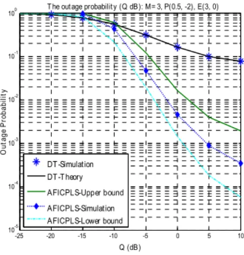
Fig. 2. Outage probability against Q(dB)

Fig. 2 presents the outage probability of the destination D of the AFICPLS and DT protocols against Q (dB) with the number of relays M=3, and the target data rate of the secondary network Rs=1 bit/s/Hz, the coordinates P(0.5, -3) and E(3, 0), (thus, dsp=2,dse=3,d3=2.5,d4=2). In Fig. 2, the outage probability of the AFICPLS protocol is less than that of the DT protocol at high Q regions (larger than -12 dB).

This is because in the high Q regions, the interference at the primary node decreases, the transmit power of the source S and relays Ri will increase. Moreover, the signal received at the destination D will increase more than that of the eavesdropper E, so that ASR at the destination D will increase. This explains why the

performance of the AFICPLS protocol is better than the DT protocol when the interference constraints increase and d

³

> d

²

. In addition, the expressions of the lower and upper bounds cover up the exact expression of the outage probability of the AFICPLS protocol (AFICPLS simulation).

-30 -25 -20 -15 -10 -5 0 5 10

10^-2 10^-1 10⁰

Q (dB)

OutageProbability

Out age probabilit y (Q dB): M= 3, 04 locat ion pairs (P, E) in Table I

L1 L2 L3 L4

그림 3. Q에 따른 정전 확률과 표 1에 나타난 P, E 노드의 04 할당

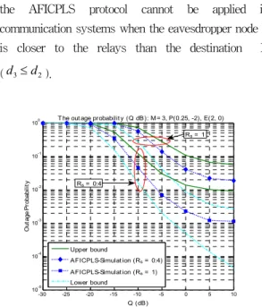
Fig. 3. Outage probability against Q (dB) with 04 location pairs of nodes (P, E) as Table 1

Notation Coordinates P and E Distances L1 (0.25, -1) (1, 0) dsp=1, dse=1,

d3=0.5, d4=1 L2 (0.25, -2) (1, 0) dsp=2, dse=1, d3=0.5, d4=2 L3 (0.25, -1) (2, 0) dsp=1, dse=2, d3=1.5, d4=1 L4 (0.25, -2) (2, 0) dsp=2, dse=2, d3=1.5, d4=2 표 1. P, E 노드의 할당

Table 1. Location pairs of nodes P and E

Fig. 3 presents the outage probability against Q (dB)

with 04 location pairs (P, E) in Table I when M=3 and

Rs=1 (bit/s/Hz). In Fig. 3, the outage probability of the

location pair L4 is best, while that of the location pair

L1 is the worst. Hence, the system performance of the

AFICPLS protocol will improve when both the primary

node P and the eavesdropper node E are further from

the secondary network. In addition, as seen in Fig. 3,

the AFICPLS protocol cannot be applied in communication systems when the eavesdropper node E is closer to the relays than the destination D ( d

³

≤ d

²

_).

-30 -25 -20 -15 -10 -5 0 5 10

10^-5 10^-4 10^-3 10^-2 10^-1 10⁰

Q (dB)

OutageProbability

T he out age probabilit y (Q dB): M= 3, P(0.25, -2), E(2, 0)

Upper bound

AFICPLS-Simulat ion (Rs= 0:4) AFICPLS-Simulat ion (Rs= 1) Lower bound

Rs= 1

Rs= 0:4

그림 4.



_가 0.4, 1(bit/s/Hz)로 고려되었을때의 Q에 따 른 정전 확률

Fig. 4. Outage probability against Q (dB) when Rs is considered at 0.4 and 1 (bit/s/Hz)

Fig. 4 presents the outage probability against Q when M=3, P (0.25, -2), E (2, 0) (thus dsp=2,dse=2,d3=1.5,d4=2) and with different target data rates of the secondary network (Rs=0.4and Rs=1 ). In Fig. 4, when Rs increases, the outage probability increases, so the performance of the system decreases.

-30 -25 -20 -15 -10 -5 0 5 10

10^-8 10^-7 10^-6 10^-5 10^-4 10^-3 10^-2 10^-1 10⁰

Q (dB)

OutageProbability

Diversit y Gain: d3= 20, P(0.25, -3)

AFI CPLS-Upper bound AFI CPLS-Simulat ion AFI CPLS-Lower bound

M = 3

M = 1

DG= 0.98 DG= 0.96

DG= 1.03

DG= 2.88 DG= 3.06

DG= 2.94

그림 5. Rs = 1(bit/s/Hz), P (0.25, -3), dsp=3, d4=3,d3=20, M =1, 3 일 때, 다이버시티 이득

Fig. 5. Diversity gain when Rs=1(bit/s/Hz), P (0.25, -3), dsp=3,d4=3,d3=20 and M =1, 3.

Fig. 5 presents the diversity gain based on the outage probabilities against (dB) when the distances from the relays Ri to the eavesdropper E (d3) move towards infinity (d3=20). In Fig. 7, the diversity gains are calculated in the rectangular region from Q= -5 dB to 5 dB of the outage probability and achieve almost full diversity corresponding to the numbers of relays M=1 and M=3. The diversity gain values of the upper bound, simulation, and lower bound of the AFICPLS protocol are very close. Hence, the secondary network achieves full diversity when the distances from the relays to the eavesdropper E (d3) move towards infinity. In addition, when the number of relays M increase, the outage probability of the AFICPLS protocol decreases; and the exact outage probability (simulated result) closely matches with the lower bound of the AFICPLS protocol in high Q regions.

V. Conclusion

In this paper, the performance of the

Amplify-and-Forward Scheme under an interference

constraint and Physical Layer Security is analyzed and

evaluated by the lower and upper bounds of the outage

probability of ASR. The best relay is selected based on

the opportunistic relay selection method in which the

end-to-end ASR is maximized. Based on the

simulation results, the performance of the proposed

protocol outperforms the direct transmission protocol,

and will improve when both the primary user and the

eavesdropper node are further from the source node

and the relays. The simulation results also show that

lower and upper expressions cover the exact

expressions of the AFICPLS protocol, and the

secondary network achieves full diversity gain when

the distances from the relays to the eavesdropper node

move toward infinity.

Appendix

A: Solving the lower bound P

^ilower

in (15) The lower bound P

^ilower

is expanded in(A.1) by detecting min formulas.

2 3

2 1 3 1

1 3

2 1 3 1

2 1

2 1 3 1

2 1

Pr , ,

2

Pr , ,

2

Pr , ,

2

Pr ,

lower i i

i sp i rp i sp i rp i

rp rp

i i

sp i rp i sp i rp i

sp rp

i i

sp i rp i sp i rp i

rp sp

sp i rp i

P m m m m

m m

m m m m

m m

m m m m

m m

m m

ω αω

ω ω ω ω θ

ω αω

ω ω ω ω θ

ω αω

ω ω ω ω θ

ω ω

⎡ ⎤

= ⎢ < < < + ⎥

⎢ ⎥

⎣ ⎦

⎡ ⎤

+ ⎢ ≥ < < + ⎥

⎢ ⎥

⎣ ⎦

⎡ ⎤

+ ⎢ < ≥ < + ⎥

⎢ ⎥

⎣ ⎦

+ ≥

_{3 1}

,

^{1 1}

2

i i

sp i rp i

sp sp

m m

m m

ω αω

ω ω θ

⎡ ⎤

≥ < +

⎢ ⎥

⎢ ⎥

⎣ ⎦

(A.1) Next, we continue the expansions for each part of the sum in (A.1), then, after some straightforward manipulations, the lower bounds P

^ilower

are obtained as

When α ≥ 2 _:

3 1 2

1 3 2 3

0

1 Pr ,

2 2

1 ( ) 1 ( ) 1 ( )

2 2

i i i

sp lower

i i sp i i rp i

rp

sp

sp rp

rp

P m m m

m

m x x

f x F m F m dx

ω ω

m

ω

α α

ω θ ω ω θ ω

α α

θ θ

∞

⎡ ⎤

= − ⎢ > + > + ⎥

⎢ ⎥

⎣ ⎦

⎧ ⎫

⎪ ⎪⎧ ⎫

= − ⎨ − + ⎬⎨ − + ⎬

⎩ ⎭

⎪ ⎪

⎩ ⎭

∫

(A.2) When α < 2 _:

1 3

3 1 1 1 2 1

2 3 1 3 3 2

2 3 1 3 3 2

Pr 2

Pr ,

2

Pr , ,

2 2

Pr , ,

2 2

sp lower

i i sp i

rp

rp rp

i i i i rp i

sp sp

sp

i rp i i sp i i

rp

sp

i rp i i i i

rp

P m m

m

m m

m m m

m m m

m m m

m

ω θ α ω

ω ω ω φ ω θ α ω

α α

ω θ ω ω θ ω ω φ

ω θ α ω ω ω ω φ

⎡ ⎤

= ⎢ < + ⎥

⎢ ⎥

⎣ ⎦

⎡ ⎤

− ⎢ > > , > + ⎥

⎢ ⎥

⎣ ⎦

⎡ ⎤

+ ⎢ < + > + < ⎥

⎢ ⎥

⎣ ⎦

⎡ ⎤

+ ⎢ < + > >

⎢⎣ ⎦ ⎥ =

⎥

3 1

1 2 3

1 2

3 1 2

3 1

0

0

( ) ( )

2

( ) 1 ( ) 1 ( )

2

( ) 1 ( ) ( )

2 2

( ) 1 ( )

2

i i

i i i

i i i

i i

sp sp

rp

rp rp

rp

sp sp

sp

sp rp

rp

sp

rp

f x F m m x dx m

m x m x

f x F m F dx

m m

m x x

f x F m F m dx

m f x F m x

m

ω ω

ω ω ω

φ φ

ω ω ω

ω ω

θ α

θ α

α α

θ θ

∞

∞

= +

⎧ ⎫⎧ ⎫

⎪ ⎪⎪ ⎪

− ⎨ − + ⎬⎨ − ⎬

⎪ ⎪⎪ ⎪

⎩ ⎭⎩ ⎭

⎧ ⎫

⎪ ⎪

+ ⎨ − + ⎬ +

⎪ ⎪

⎩ ⎭

⎧ ⎫

⎪ ⎪

+ ⎨ − ⎬

⎪⎩ ⎭

∫

∫

∫

2 2

( )

2

i rp

F

_ω

m x

φ

θ α

∞

⎪ +

∫

(A.3) The result of (A.2) and (A.3) is solved as in (17) and (18), where f

_ωai

^{( )} x = λ

a

e

^−λax

^, a ∈ { } ^1,3 _{are the}

probability density functions (PDFs) of ω ;and

^1a

( ) 1

^b

,

bi

F_ω x

= −

e^−λx

^b∈ { ^1,2,3 } _{are the} cumulative distribution functions (CDFs) of ω ; and

^1b

( )

1

m

sp

1 2

φ = θ − α _, φ

2

= m

rp

θ ( 1 − α 2 ) _.

B: Solving the upper bound P

^iupper

in(16) The upper bound P

^iupper

is expanded as

2 3

2 1 3 1

1 3

2 1 3 1

2 1

2 1 3 1

2 1

Pr , ,

2

Pr , ,

2

Pr , ,

2

Pr ,

upper i i

i sp i rp i sp i rp i

rp rp

i i

sp i rp i sp i rp i

sp rp

i i

sp i rp i sp i rp i

rp sp

sp i rp i

P m m m m

m m

m m m m

m m

m m m m

m m

m m m

ω αω

ω ω ω ω θ

ω αω

ω ω ω ω θ

ω αω

ω ω ω ω θ

ω ω

⎡ ⎤

= ⎢ < < < + ⎥

⎢ ⎥

⎣ ⎦

⎡ ⎤

+ ⎢ ≥ < < + ⎥

⎢ ⎥

⎣ ⎦

⎡ ⎤

+ ⎢ < ≥ < + ⎥

⎢ ⎥

⎣ ⎦

+ ≥

_{3 1}

,

^{1 1}

2

i i

sp i rp i

sp sp

m m m

ω αω

ω ω θ

⎡ ⎤

≥ < +

⎢ ⎥

⎢ ⎥

⎣ ⎦

(B.1) We perform some straightforward manipulations so that finally, P

^iupper

is obtained and calculated as

(

1 2

)

3

1 2 3

2 3

3 2 1

1 Pr 2 2 , 2 2

1 2 2

sp rp

sp i upper

i i sp i rp i

rp

m m

sp rp

P m m m

m e

m m

θ λ λ

ω θ α ω ω θ αω

λ

λ αλ α λ

− +

⎡ ⎤

= − ⎢ > + > + ⎥

⎢ ⎥

⎣ ⎦

= − + +

(B.2)

References

[1] Sang-Young Park; Hyung-Yun Kong, "Multihop Transmission in Cognitive Underlay Network Over Rayleigh Fading Channels", Journal of the Institute of Webcasting, Internet and Telecommunication (IWIT), vol.12, no.6, pp. 291-296, Dec. 2012.

[2] Hussain, S.I.; Abdallah, M.M.; Alouini, M.-S.;

Hasna, M.; Qaraqe, K., "Performance Analysis of Selective Cooperation in Underlay Cognitive Networks over Rayleigh Channels", IEEE 12th International Workshop on Signal Processing Advances in Wireless Communications, p.116-120, 2011.

[3] Nam-Soo Kim, "Performance of DOT Relay System with MRC/GSC receiver in Rayleigh Fading Channels", Journal of the Institute of Webcasting, Internet and Telecommunication(IWIT), vol. 12, no.

5, pp. 11-16, Oct. 2012.

[4] Nam-Soo Kim, "Incremental Best Relay Selection System with Outdate CSI in Rayleigh Fading Channels", Journal of the Institute of Webcasting, Internet and Telecommunication(IWIT), vol. 12, no.

5, pp. 17-23, Oct. 2012.

[5] Minghua Xia; Aissa, S., "Cooperative AF Relaying in Spectrum-Sharing Systems: Outage Probability Analysis under Co-Channel Interferences and Relay Selection", IEEE Transactions on Wireless Communications, vol. 60, no. 11, pp. 3252–3262, 2012.

[6] Lun Dong; Zhu Han; Petropulu, A.P.; Poor, H.V.,

"Improving Wireless Physical Layer Security via Cooperating Relays", IEEE Transactions on Signal Processing, vol 58, no. 3, pp.1875-1888, 2010.

[7] Xiaojun Sun; Wei Xu; Ming Jiang; Chunming Zhao,

"Opportunistic Selection for Decode-and-Forward Cooperative Networks with Secure Probabilistic Constraints", Wireless Personal Communications, vol. 70, no. 4, pp. 1633-1652, June 2013.

저자 소개

공 형 윤(정회원)

∙1989년 2월 : New York Institute of Technology(미국) 전자공학과 학사

∙1991년 2월 : Polytechnic University (미국) 전자 공학과 석사

∙1996년 2월 : Polytechnic University (미국) 전자 공학과 박사

∙1996년～1996년 : LG전자 PCS팀장

∙1996년～1998년 : LG 전자 회장실 전략 사업단

∙1998년～현재 : 울산대학교 전기전자정보시스템공학부 교수 <주관심분야> 모듈레이션, 채널 부호화, 검파 및 추정 기술,

협력통신, 센서네트워크

Pham Ngoc Son(학생회원)

∙2005년 2월 : Ho Chi Minh City University of Technology 학사

∙2009년 2월 : Ho Chi Minh City University of Technology 석사

∙2012년 3월 ～ 현재 : 울산대학교 전 기공학부 박사 과정

<주관심분야> 협력통신, 인지기술, 물리 계층 보안, 결합 기

술, 무선 센서 네트워크