Three-Dimensional Image Reconstruction from Compton Scattered Data Using the Row-Action Maximum Likelihood Algorithm

(1)

Ⅰ. 서 론

(Compton)

ECT (Emission Computed Tomography) PET (Positron Emission Tomography) SPECT (Single-Photon Emission Computed

Tomography) ECT (scatterer)

(absorber)

.[1]

(electronic collimation)

(mechanical collimation)

SPECT .

(multitracer imaging) .[2,3]

.

3

이미노¹, 이수진¹, Van-Giang Nguyen¹, 김수미², 이재성²

1 , ²

Three-Dimensional Image Reconstruction from Compton Scattered Data Using the Row-Action Maximum Likelihood Algorithm

Mi No Lee¹, Soo-Jin Lee¹, Van-Giang Nguyen¹, Soo Mee Kim², Jae Sung Lee²

1Department of Electronic Engineering, Paichai University, Daejeon, Korea

2Department of Nuclear Medicine and Interdisciplinary Program in Radiation Applied Life Science Major Seoul National University College of Medicine, Seoul, Korea

(Received November 26, 2008. Accepted February 12, 2009)

Compton imaging is often recognized as a potentially more valuable 3-D technique in nuclear medicine than conventional emission tomography. Due to inherent computational limitations, however, it has been of a difficult problem to reconstruct images with good accuracy. In this work we show that the row-action maximum likelihood algorithm (RAMLA), which have proven useful for conventional tomographic reconstruction, can also be applied to the problem of 3-D reconstruction of cone-beam projections from Compton scattered data. The major advantage of RAMLA is that it converges to a true maximum likelihood solution at an order of magnitude faster than the standard expectation maximiation (EM) algorithm. For our simulations, we first model a Compton camera system consisting of the three pairs of scatterer and absorber detectors placed at x-, y- and z-axes, and generate conical projection data using a software phantom. We then compare the quantitative performance of RAMLA and EM reconstructions in terms of the percentage error. The net conclusion based on our experimental results is that the RAMLA applied to Compton camera reconstruction significantly outperforms the EM algorithm in convergence rate; while computational costs of one iteration of RAMLA and EM are about the same, one iteration of RAMLA performs as well as 128 iterations of EM.

Compton camera, emission tomography, statistical image reconstruction, maximum likelihood estimation, maximum a posteriori estimation

Corresponding Author : ^이수진

(302-735) 대전광역시 서구 연자 1길 14 배재대학교 전자공학과 Tel : +82-42-520-5711 / Fax : +82-42-520-5687 E-mail : [email protected]

본 연구는 과학기술부 및 과학재단의 지원을 받아 2008년도 원자력기초공동연 구소 (해상도 5mm급 컴프턴 카메라의 실증과 응용)를 통해 수행되었음.

(2)

PET SPECT .

.

[4]

[5-10]

[11,12] .

.



.

(maximum likelihood expectation maximization, MLEM)[13,14]

. Browne De Pierro RAMLA (row-action maximum likelihood

algorithm) [15] (row-action) (like-

lihood)

ML (maximum likelihood)

.

RAMLA SPECT PET

. RAMLA

MLEM

.

Ⅱ. 컴프턴 영상시스템의 투사과정

1

. ,

, .

(1)

,

 _ _ _

 _ _ _, _

_ 

.^__

Image space Scatterer Absorber

그림 1. 컴프턴 카메라 시스템에서 타원추 표면을 따른 투사데이터의 형성. Fig. 1. Formation of conical projection data in a Compton camera system.

(3)

    __



__

(1)

1



. ,



.

 , , 

.





.

^ ^ ^{ }^ ⁽²⁾

(2) 

.

__ _.

_ ω

(solid angle)

(differential cross-section) Klein-Nishina

.[16] _

, , 

.

(ellipse-stacking method, ESM) (ray-tracing method, RTM) .[17,18]

3 x-y

-

_ 2

. 1

.

_

(chord length) .[19]

_ .

Ⅲ. 최대우도 방법을 사용한 영상재구성 알고리즘

ECT (2)

(deterministic)

. (2)

. (analytic)

(linear algebraic) . ECT

(filtered back-projection, FBP) [20]

(algebraic reconstruction technique, ART)[21] . FBP SPECT

PET

(Radon transform)

. ART

(2) N

M .

(3)

(iterative) .

 ^{ }    

^^

^ ^

 (3)

(3) 

   . 

(relaxation) . (3)

.

PET/SPECT

.

(4)

(Poisson) .

(4) .

      ^    _

(4)

(4) ^ 

,  

.



 

, 

ML . , (5)



 .

  



    (5)

(maximum likelihood expectation maximization,

MLEM)[13,14] . MLEM

“

”(incomplete)

“ ”(complete)

 .

  



   

 

 _      ⁽⁶⁾ 2

. ,

. C EM

.

MLEM E-

M- (7) .

 ^{ } 

^

 ^^ ^



(7)

(7) ^ ^ ^MLEM

^ ^ ^ ^

. MLEM

(7) 

FBP ART

. MLEM

(ill-posed problem) ML

.

EM Hudson Larkin

OS-EM (ordered subsets EM)[22]

MLEM

. OS-EM EM

(susbset) ( (block))

. 

 .

MLEM .

RAMLA OS-EM

(gradient descent) ML

(relaxation parameter) , ART

MLEM (row action)

ML .

(5)

 ^{ }      





^^^ ^ ^{ }^^



^ ⁽⁸⁾

(8) , 

,  . 

(relaxation) 

   ≤  . (8) OS

RAMLA (9) .

^{  } ^{   }  ^{   }

_∈^





^^^ ^^{    } ^{ }^^



^ ^    ⁽⁹⁾

_∈^ (10)

   ≤    ≠ ₍₁₁₎

^{ }  ^{ }, ^{  }  , .

. (10)



 (11) , 

 . (9)

(12)  (13)

.[23,24]

  _∈^ ⁽¹²⁾

^{  } ^{   }  

^{   }

_∈^





^^^ ^^{    } ^{ }^^



^ ^

(13)



. RAMLA 

. (14)

0  . 

 0 .

   

 (14)

(14) 

.  .

Ⅳ. 실험 및 결과

A. 모의실험 모의실험 모의실험 모의실험 환경 환경 환경 환경 및 및 및 소프트웨어 및 소프트웨어 소프트웨어 모형 소프트웨어 모형 모형 모형

1

5cm×5cm 16×16

. -

- 5cm

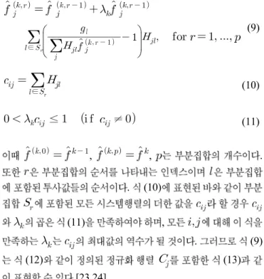
(a) (b) (c) (d)

(e) (f) (g) (h)

250 200 150 100 50

그림 2. 잡음이 포함되지 않은 투사 값으로부터 재구성된 x-y평면 영상: (a) 소프트웨어 모형; (b) SBP; (c) MLEM (8 iterations); (d) MLEM (32 iterations); (e) RAMLA (σ=2, 8 iterations); (f) RAMLA (σ=2, 32 iterations); (g) RAMLA (σ=20, 8 iterations); (h) RAMLA (σ=20, 32 iterations).

Fig. 2. x-y plane images reconstructed from noiseless projections: (a) software phantom; (b) SBP; (c) MLEM (8 iterations); (d) MLEM (32 iterations); (e) RAMLA (σ=2, 8 iterations); (f) RAMLA (σ=2, 32 iterations); (g) RAMLA (σ=20, 8 iterations); (h) RAMLA (σ=20, 32 iterations).

(6)

 ≤  ≤  2.5˚ 32

. 1

(view angle) 180˚

x- , y- , z- 3 .

. 10×10×10cm³ 64×64×64 3

6

1:4:6:8 . ( 2(a) )

RAMLA

ML MLEM

SBP (simple back-projection)

. RAMLA MLEM ML

. ML .

.

B. 영상재구성 영상재구성 영상재구성 영상재구성 결과결과결과결과

2~7 SBP, MLEM, RAMLA 3 2, 3, 4

(a) (b) (c) (d)

(e) (f) (g) (h)

250 200 150 100 50

그림 3. 잡음이 포함되지 않은 투사 값으로부터 재구성된 y-z평면 영상: (a) 소프트웨어 모형; (b) SBP; (c) MLEM (8 iterations); (d) MLEM (32 iterations); (e) RAMLA (σ=2, 8 iterations); (f) RAMLA (σ=2, 32 iterations); (g) RAMLA (σ=20, 8 iterations); (h) RAMLA (σ=20, 32 iterations).

Fig. 3. x-y plane images reconstructed from noisy projections: (a) software phantom; (b) SBP; (c) MLEM (8 iterations); (d) MLEM (32 iterations); (e) RAMLA (σ=2, 8 iterations); (f) RAMLA (σ=2, 32 iterations); (g) RAMLA (σ=20, 8 iterations); (h) RAMLA (σ=20, 32 iterations).

(a) (b) (c) (d)

(e) (f) (g) (h)

250 200 150 100 50

그림 4. 잡음이 포함되지 않은 투사 값으로부터 재구성된 x-z평면 영상: (a) 소프트웨어 모형; (b) SBP; (c) MLEM (8 iterations); (d) MLEM (32 iterations); (e) RAMLA (σ=2, 8 iterations); (f) RAMLA (σ=2, 32 iterations); (g) RAMLA (σ=20, 8 iterations); (h) RAMLA (σ=20, 32 iterations).

Fig. 4. x-y plane images reconstructed from noisy projections: (a) software phantom; (b) SBP; (c) MLEM (8 iterations); (d) MLEM (32 iterations); (e) RAMLA (σ=2, 8 iterations); (f) RAMLA (σ=2, 32 iterations); (g) RAMLA (σ=20, 8 iterations); (h) RAMLA (σ=20, 32 iterations).

(7)

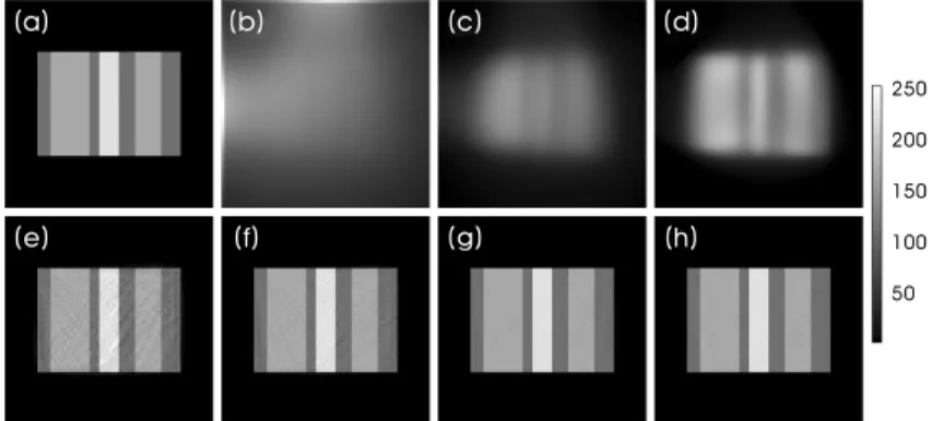
, 5, 6, 7

. 2 5 x-y , 3

6 y-z , 4 7 x-z .

(a) (b)

, (c) (f) MLEM (c)

8 , (f) 32 . (d), (e),

(a) (b) (c) (d)

(e) (f) (g) (h)

250 200 150 100 50

그림 5. 잡음이 포함된 투사 값으로부터 재구성된 x-y^{평면 영상}: (a) ^{소프트웨어 모형}; (b) SBP; (c) MLEM (8 iterations); (d) MLEM (32 iterations); (e) RAMLA (σ

=0.1, 8 iterations); (f) RAMLA (σ=0.1, 32 iterations); (g) RAMLA (σ=0.2, 8 iterations); (h) RAMLA (σ=0.2, 32 iterations).

Fig. 5. x-y plane images reconstructed from noisy projections: (a) software phantom; (b) SBP; (c) MLEM (8 iterations); (d) MLEM (32 iterations); (e) RAMLA (σ

(a) (b) (c) (d)

(e) (f) (g) (h)

250 200 150 100 50

그림 6. 잡음이 포함된 투사 값으로부터 재구성된 y-z^{평면 영상}: (a) ^{소프트웨어 모형}; (b) SBP; (c) MLEM (8 iterations); (d) MLEM (32 iterations); (e) RAMLA (σ

(a) (b) (c) (d)

(e) (f) (g) (h)

250 200 150 100 50

그림 7. 잡음이 포함된 투사 값으로부터 재구성된 x-z^{평면 영상}: (a) ^{소프트웨어 모형}; (b) SBP; (c) MLEM (8 iterations); (d) MLEM (32 iterations); (e) RAMLA (σ

(8)

(g), (h) RAMLA 2, 3, 4

(d), (g) (14) σ=2, (e), (h) σ=20 ,

5, 6, 7 (d), (g) σ=0.1, (e), (h) σ=0.2 . (d), (e) 8 , (g), (h) 32

.

(14) σ

8 . 1

PE (percentage error, PE) PE  (15)

,  _.

 ^^^ ^{ }^^^^ ^^{× } ⁽¹⁵⁾

9

PE .

2~7 (b) SBP

. ( 3, 4, 6, 7 (b) ) 1 SBP PE PE

SBP

.

MLEM RAMLA

Number of lterations

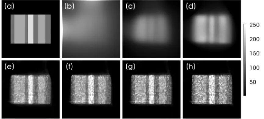
1 0.9 0.8 0.7 0.6 0.5 0.4 0.3 0.2 0.1

Lambda

0 5

0

10 15 20 25 30

σ = 0.1 σ = 0.2 σ = 2.0 σ = 20

그림 8.반복연산 횟수의 증가 및 σ에 따른 완화파라미터. Fig. 8. Relaxation parameter versus number of iterations for various σ's.

noiseless noisy

Algorithm

Iterations SBP MLEM RAMLA

(σ=2)

RAMLA

(σ=20) SBP MLEM RAMLA

(σ=0.1)

RAMLA (σ=0.2) 1

55.04

×10⁷

84.83 25.92 25.10

55.03

×10⁷

84.83 37.67 34.03

2 78.20 15.45 13.06 78.20 27.84 25.77

4 66.47 10.79 7.49 66.50 25.28 24.19

8 52.85 7.89 4.38 52.86 24.04 24.03 (6^th)

16 43.20 3.00 2.61 43.20 23.46 24.62

32 35.79 4.78 1.59 35.80 23.8 (35^th) 25.47

64 29.67 3.94 1.03 29.73 23.36 26.50

128 24.43 3.32 0.72 24.73 23.61 27.61

표 1. SBP, MLEM, RAMLA 영상의 퍼센티지 오차

Table 1. Percentage errors of SBP, MLEM, and RAMLA reconstructions

(9)

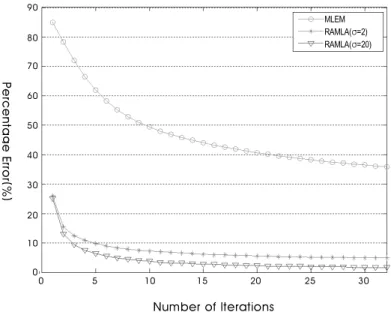
PE

RAMLA . RAMLA MLEM

. 9 PE

RAMLA MLEM

. RAMLA

8 σ

.

PE .

RAMLA

.

. .

1    35 ,

   6 .

5, 6, 7 (c) (d) MLEM

. MLEM RAMLA

128 PE

.

Ⅴ. 고찰 및 결론

RAMLA SBP

MLEM , .

SBP MLEM RAMLA

, MLEM 128 1

RAMLA PE .

RAMLA MLEM

. RAMLA

.

RAMLA .

(ill-posed problem)

(stabilizer) (regularizer) (well-posed problem)

(maximum a posteriori, MAP)

. RAMLA MAP

BSREM (block sequential regularized EM)[25]

. (prior probability)

MAP

Number of lterations

90

Percentage Error(%)

0 5

0 10 15 20 25 30

MLEM RAMLA(σ=2) RAMLA(σ=20) 80

70 60 50 40 30

20 10

그림 9. MLEM, RAMLA (σ = 2) and RAMLA(σ = 20)의 반복연산 횟수에 따른 퍼센티지 오차. Fig. 9. Percentage error versus number of iterations for MLEM, RAMLA (σ = 2) and RAMLA (σ = 20).

(10)

.

참고문헌

[1] M. Singh, “An electronically collimated gamma camera for single photon emission computed tomography: Part1 and 2”, Med. Phys., vol. 10, no. 4, pp. 421-427, 1983.

[2] Y. F. Yang, Y. Gono, S. Motomura, S. Enomoto, and Y. Yano, “A compton camera for multi-tracer imaging”, IEEE Trans. Nucl.

Sci., vol. 48, pp. 656-661, 2001.

[3] S. Motomura, H. Takeici, R. Hirunuma, H. Haba, K. Igarashi, S.

Enomoto, Y. Gono, Y. Yano, “Gamma-ray Compton imaging of multitracer in bio-samples by strip germanium telescope”, IEEE Nuclear Science Symposium and Medical Imaging Conference Record, vol. 4, pp. 2152-2154, 2004

[4] R. W. Todd, J. M. Nightingale, and D. B. Everett, “A proposed Gamma camera”, Nature, vol. 251, pp. 132-134, 1974.

[5] R. Basko, G. L. Zeng, and G. T. Gullberg, “Application of spherical harmonics to image reconstruction for the Compton camera”, Phys. Med. Biol. vol. 43, pp. 887-894, 1998.

[6] L. C. Parra, “Reconstruction of cone-beam projections from Compton scattered data”, IEEE Trans. Nucl. Sci., vol. 47, pp.

1543-1550, 2000.

[7] T. Tomitani and M. Hirasawa, “Image reconstruction from limited angle Compton camera data”, Phys, Med. Biol., vol. 47, pp. 1009-1026, 2002.

[8] M. Hirasawa and T. Tomitani, “An analytical image reconstruction algorithm to compensate for scattering angle broadening in Compton cameras”, Phys. Med. biol., vol. 48, 1009-1026, 2003.

[9] B. Smith, “Reconstruction methods and completeness conditions for two Compton data models”, J. Opt. Soc. Am. A, vol. 22, no. 3, pp. 445-459, 2005.

[10] D. Xu, Z. He, “Filtered back-projection in 4π Compton imaging with a single 3D position sensitive CdZnTe detector”, IEEE Trans. Nucl. Sci., vol 53, no. 5, pp. 2787-2793, 2006.

[11] T. Hebert, R. Leahy, and M. Singh, “Three-dimensional maximum-likelihood reconstructin for a electronically collimated single-photon-emission imaging system”, J. Opt. Soc. Am., A7, pp. 1305-1313, 1990.

[12] A. C. Sauve, A. O. Hero , W. L. Rogers, S. J. Wilderman, and N. H. Clinthorne, “3D image reconstruction for Compton SPECT

camera model”, IEEE Trans. Nucl. Sci., vol. 46, pp. 2075-2084, 1999.

[13] L. A. Shepp and Y. Vardi, “Maximum likelihod reconstruction for emission tomography”, IEEE Trans. Med. Imaging, vol. 1, pp.

113-122, 1982.

[14] K. Lange and R. Carson, “EM reconstruction algorithms for emission and transmission tomography”, J. Comput. Assist.

Tomog., vol. 8, pp. 306-316, 1984.

[15] J. Browne and A. D. Pierro. “A Row-Action Alternative to The EM Algorithm for Maximizing Likelihoods in Emission Tomography,” IEEE Trans. Med. Imaging, vol. 15, pp. 687 699, 1996.

[16] O. Klein and Y. Nishina, “Experimental Study of the Compton Effect at 1.2 Mev”, Phys. Rev., vol. 76, pp. 1269-1270, 1949.

[17] S. M. Kim, J. S. Lee, M. N. Lee, J. H. Lee, C. S. Lee, C. H. Kim, D. S. Lee, S. J. Lee, “Two approaches to implementing projector- backprojector pairs for 3D reconstruction from Compton scattered data”, Nuclear Instruments & Methods in Physics Research A, vol. 571, pp. 255-258, 2007.

[18] M. N. Lee, S. -J. Lee, S. M. Kim, J. S. Lee, “Ellipse-Stacking Methods for Image Reconstruction in Compton Cameras”, J.

Biomed. Eng. Res. vol. 28, no. 4, pp. 520-529, 2007.

[19] Siddon R. L., “Fast calculation of the exact radiological path for a three-dimensional CT array,” Med. Phys., vol. 12, pp. 252-255, 1985

[20] A. Rosenfeld and A. C. Kak, Digital Picture Processing, volume 1, Academic Press, New York, NY, 1982.

[21] G. T. Herman and L. B. Meyer, “Algebraic reconstruction techniques can be made computationally efficient “ IEEE Trans.

Med. Imaging, vol. 12, pp. 600-609, 1993.

[22] H. M. Hudson and R. S. Larkin, “Accelerated image reconstruction using ordered subsets of projection data”, IEEE Trans.

Med. Imaging, vol. 13, pp. 601-609, 1994.

[23] E. Tanaka and H. Kudo “Subset-dependent relaxation on block- iterative algorithms for image reconstruction in emission tomography”, Phys. Med. biol., vol. 48, pp. 1405-1422, 2003.

[24] A. Fukano, T. Nakayama and H. Kudo “Performance evaluation of relaxed block-iterative algorithms for 3-D PET reconstruction”, IEEE Nuclear Science Symposium Conference and Medical Imaging Conference Record, vol. 5, pp. 2830-2834, 2004.

[25] A. D. Pierro and M. E. B. Yamagishi, “Fast EM-like methods for maximum ‘A Posteriori’ estimates in Emission tomography”, IEEE Trans. Med. Imaging, vol. 20, no. 4, pp. 280-288, 2001.