Numerical Analysis of Piezocone Test using Modified Cam-Clay Model

Numerical Analysis of Piezocone Test using Modified Cam-Clay Model

Modified Cam－Clay Model을 이용한 피에조콘 시험의 수치해석

Kim, Dae-Kyu*ㆍLee, Woo-Jin**

김대규ㆍ이우진

요 지

본 연구에서는 가장 널리 사용되고 있는 지반모델인 Modified Cam-Clay 모델을 이용하여 피에조콘 관입 및 소

산시험의 수치해석을 수행하였다. Modified Cam-Clay 모델 및 관련 유한요소 식들을 피에조콘 관입의 대변형 현상을 고려하기 위하여 Updated Lagrangian frame에서 formulation 하였다. 유한요소 해석 결과 얻어진 콘 관입저항치, 간극수압 및 소산곡선을 양산지역 현장 시험결과와 비교 분석하였다. 수치해석 결과는 시험결과와 비교적 잘 부합하는 것으로 고찰되었으나 보다 현실에 근접한 simulation을 위하여 연속적인 깊은 관입의 적절한 수치해석적 modeling이 요구되는 것으로 고찰되었다.

주요어 : Modified Cam-Clay model, 피에조콘, Updated Lagrangian formulation, 간극수압소산

Abstract

In this study, the numerical analysis of piezocone penetration and dissipation tests has been conducted using the Modified Cam-Clay model, which is generally used in soil mechanics. The Modified Cam-Clay model and related mathematical equations in finite element derivation have been formulated in the Updated Lagrangian reference frame to take the large displacement and finite strain nature of piezocone penetration into consideration. The cone tip resistance, the pore water pressure, and the dissipation curve obtained from the finite element analysis have been compared and investigated with the experimental results from piezocone penetration test performed in Yangsan site. The numerical results showed good agreement with the experimental results; however, the better numerical simulation of the continuous and deep penetration needs further research.

Keywords : Modified Cam-Clay model, Piezocone, Updated Lagrangian formulation, Dissipation

* 정회원․고대부설 방재과학기술연구센터 선임연구원

** 정회원․고려대학교 토목환경공학과 부교수

···

···

한국지반환경공학회 논문집 제2권 제3호 2001년 9월 pp. 89~99

`50

1. Introduction

The piezocone penetration test are now becoming a very popular and important tool for site characterization and ground contaminant study since it is relatively simple and fast; furthermore, many engineering properties can be obtained from the direct test results, i.e., cone tip resistance, pore water pressure, and sleeve friction. The reliability of the test results are, however, often influenced by many factors like soil characteristics, testing practice, and so on. To get more accurate results, many interpretation methods have been proposed, namely, semi-empirical approach, bearing capacity models, cavity expansion theory, strain path method, and numerical analysis. Finite element method among them has become an important method to analyze the complex cone penetration mechanism considering many influencing factors (Deborst and Vermeer, 1984; Kiousis et al., 1988; Sandven, 1990; Teh and Houlsby, 1991; Van den Berg et al., 1994;

Abu-Farsakh et al., 1997). It is needless to say that the choice of a proper soil model is decisively important in numerical analysis. Abu-Farsakh et al. (1997) conducted a finite element analysis of piezocone penetration test using the Modified Cam-Clay model, which is most generally used in geotechnical engineering, and Updated Lagrangian formulation to capture large displacement and finite strain nature of piezocone penetration mechanism. The numerical results were compared with experimental results performed using calibration chamber test system. Their work showed good results under well controled condition;

however, it is in doubt if the results of the finite element analysis would well match the results from field test.

In this study, the finite element analysis of piezocone penetration and dissipation tests has been performed using the Modified Cam-Clay model based on Abu-Farsakh et al. (1997). The results have been compared with the experimental results of the field test conducted in Yangsan site. The numerical formulation, the field test, and the numerical and experimental results are described in following sections.

2. Numerical Formulation

All mathematical equations adopted in this study including the Modified Cam-Clay model were formulated in the Updated Lagrangian reference frame to take large displacement and finite strain nature of piezocne penetration mechanism into account. This section briefly describes the numerical formulation based on Abu-Farsakh et al. (1997).

In the Updated Lagrangian formulation, it is postulated that a body occupies a volume V

0

, V

n

, V

n+1

at load increments 0, n, and n+1, respectively, corresponding to time t

^o

, t

ⁿ

, and t

ⁿ⁺¹

in the fixed cartesian coordinate system, and all quantities in the n+1 configuration are determined with respect to the previous n configuration. The reference configuration is updated after each incremental step. For example,

n+1 referred to the n configuration. The superscript s or ' denotes the quantities in 'effective' concept in the following development,

For finite deformations, elastoplastic constitutive equation for the solid skeleton is assumed to be (Voyiadjis and Kattan, 1989)

abcd ^s cd '

ab = D d

σ ^ο

(1)

where

ο '

σ ab

is effective corotational stress rate tensor, D is elastoplastic stress-strain matrix.

Spatial strain rate tensor d

^s

is given by

( ^s c , a )

s c , a s

ac 2

d = 1 ν + ν

(2)

where ν

^s

is velocity of solid particle. Effective corotational stress rate tensor

ο '

σ ab

is assumed to be

^{σ ' ab = σ ' ab − W ac ∗ s σ ' cd + W cb ∗ s σ ' ac}

• ο

(3)

'' s ac s ab s

ac W W

W ^∗ = −

(4)

( ^s c , a )

s c , a s

ac 2

W = 1 ν − ν

AB 1 n

n S

+

is the second Piola-Kirchhoff stress tensor at

where

σ • ^' _ab

is effective Cauchy stress rate tensor,

^{σ ' ac}

is effective Cauchy stress tensor, ^W

^{ac s ∗}

is modified spin tensor, and

^{W ac s ''}

is plastic spin tensor. The relation between Cauchy stress tensor

^{n + 1 σ ab}

and second Piola-Kirchhoff stress tensor

^{n + n 1 S AB}

is given by

AB 1 n

n s

B , b s

A , a s 1 ab 1

n ⁺ σ = J ⁻ X X ⁺ S ^{n +} _n ¹ S _AB = J ^s X ^s _{A , a} X ^s _{B , b} ^{n + 1} σ _ab

(5)

where

^{J s}

is corresponding Jacobian for solids and

s A ,

X a

is deformation gradient expressed as

s A n

s a 1 n

s A n

s s a

A ,

a X

X X

X Z

∂

= ∂

∂

= ∂ ⁺

(6)

and spatial strain rate tensor d

^s

is related to the material strain rate tensor

ε ^{• s}

by

ε •

= ^s _{c , C} ^s _{d , D} ^s _CD

s

cd X X

d

(7)

Using the above equations and after manipulation, the following relations are obtained.

ab w s

b , B s

a , A s CD ABCD

ab D J X X P

S ^• = ^∗ ε ^• + ^• δ

(8)

cd ab w cd s ' ab bd s ' ac ad s ' cb ABCD

ABCD [ D P

D ^∗ = − σ δ − σ δ + σ δ + ^• δ δ

^{− 2 P w δ ac δ bd ]( J s X s A , a X s B , b X s C , c X s D , d )}

(9)

where P

w

is pore water pressure.

Virtual work equation in Updated Lagrangian formulation is given by (Bathe, 1990)

( ) ^{d V R}

S ^{n n 1}

V AB

1 n

n AB 1 n

n

n

+ +

+ δ ε =

∫

(10)

AB n AB n 1 n

n ε = e + η

+

(11)

)

u u 2 (

e _AB 1 _{n A , B n B , A}

n = + ( u u )

2 1

B , K n A , K n AB

n η = +

(12) where u is displacement vector. Second Piola- Kirchhoff stress tensor

^{n + n 1 S AB}

at n+1 referred to the n configuration is related to Cauchy stress tensor

^{n σ AB}

by

AB n AB n AB 1 n

n S = σ + ∆ S

+

(13)

Using Eqs. (10), (11), and (13), and

^{∆ n S AB}

expressed using Eqs. (8) and (9), the following virtual work equation is obtained.

(

n CD n CD

)

n AB ⁿ

V D ABCD e e dV

n ∆ + ∆ η δ

∫ ^∗

n AB n CD

V

D

ABCD n

e dV

n

∆ δ η

+

∫ ^∗

( ) n AB ⁿ

V w AB

n ' AB

n P dV

n σ + δ δ η

+ ∫

(

n AB n AB

)

ⁿ

V ab w

s b , B s

a , A

s X X P e dV

n J δ ∆ δ + δ η

+ ∫

( ) n AB ⁿ

V w AB

n ' AB n 1

n

R−

_n

σ + P δ δ e dV

=

⁺ ∫

(14)

Theory of mixtures was used to explain the behavior of soils as a multiphase medium (Prevost, 1980). In theory of mixtures, soil is considered as a mixture of multiphase deformable medium of solid grains and water when saturated. Solid grain and water are respectively regarded as a continuum and as a fluid.

The final coupled equation in theory of mixtures is derived using the law of conservation of mass and a certain flow law of water through the voids. The coupled equation in theory of mixtures in Updated Lagrangian formulation is obtained as (Kiousis et al., 1988; Voyiadjis and Abu-Farsakh, 1997)

, 0 ,

1 1

1 − =

∂

∂

∂

− ∂

− −

− •

⎥ ⎥

⎦

⎤

⎢ ⎢

⎣

⎡

⎟ ⎟

⎠

⎞

⎜ ⎜

⎝

⎛

B B w X B

P w s

A X a ws K AB w n w

X D s

a X D s C ij s C ij J s ij s C ij

J s ρ

ε γ

(15)

s k,j s k,i s

ij X X

C =

^{b b = X s b , B B B}

(16)

Where b is body force vector,

K ^ws

is permeability applied loads and surface tractions, V is volume,

^{n +1 n ε}

is total strain, and it is decomposed into linear strain

^{n +1 n ε}

is total strain, nonlinear strain

^{n η AB}

.

where

^{n+ 1} R

is external virtual work due to the

tensor in m/sec,

^{γ w}

is unit weight of water, and

^{ρ w}

is intrinsic mass density of the water. Soil porosity n

^w

is updated from at n configuration to at n+1 configuration using Jaccobian of solid grains

J ^s

.

^w n ^s w

1 n

J 1 n 1

n

1 =

−

− ₊

(17)

Eqs. (14) and (15) are implemented into a finite element formulation.

u= h⋅U

^{P w = N ⋅ W}

X ^W P

B , B

w = N

∂

∂

(18)

The above finite element discretization is used for displacement u and pore water pressure P

w

. h is displacement shape function, N is pore water pressure shape function, U is nodal displacement, and W is nodal pore water pressure. The variation of linear and nonlinear strains are given by

U e = _L ⋅ δ

δ B

^{δη B = NL ⋅ δ U}

(19)

where B

L

and B

NL

are linear and nonlinear strain-displacement matrices. Using Eqs. (14) and (19), the following expression is obtained.

Φ

Ω _n

n

n K ∆ U + ∆ W =

(20)

In Eq. (20), the elastoplastic stiffness matrix

^{n K}

is expressed as

s n T NL n NL n L n

n K = K + K + K + K

(21)

V ^{n L d n V}

T L n L

n K ⁼ ∫ n B ^⋅ D ^{∗ ⋅} B

^{n K NL}

⁼

∫ ^{n V n B T L}

^⋅

^{D ∗}

^⋅

^{n B NL}

^d

ⁿ

^V (22)

V d ⁿ

V n NL s

n ^{K =} ∫ n ^{C ⋅ n C NL = n B ∗ NL T ⋅ n σ ⋅ n B ∗ NL}

(23) where

^{n K L}

is linear stiffness matrix,

^{n K NL}

is nonlinear matrix.

^{n K s}

is nonlinear geometric stiffness matrix, and

^{n C NL}

is nonlinear matrix. The coupling matrix

^{n Ω}

in Eq. (20) is expressed as

( )

^{d V}

X X

J

T ab ⁿ

NL n T L V n

s b , B s

a , A s

n

^Ω=

∫ n B

+

B N N = m N

(24)

where

m

^T

={1 1 0} for two dimension

m

^T

={1 1 1 0 0 0} for three dimension (25) In Eq. (20),

(26) Eq. (15) is expressed in finite element form thorugh Galerkin's weighed residual method and Green's theory as

Π

Ψ

Ω ^T _{n n}

n ∆ U + δ t ∆ W =

−

(27)

where

V d N N K C n C

J , A , B ⁿ

ws AB n s ij s ij w w

V s n

1 1 n

−

−

= ∫ γ

Ψ

(28)

A d P q W t

t

w ⁿ

S n n n

n

^Π=δ

^G

^{−δ Ψ −}

∫ n

(29)

V d N N K C C n

J , A , B ⁿ

ws AB n s ij s ij w v

s ^{1 1}

N

−

∫ −

−

G =

(30)

^{∆ U = U n + 1 − U n}

^{∆ W = W n + 1 − W n}

(31)

where

^{∆ U}

is incremental nodal displacement,

^{∆ W}

is incremental nodal excess pore water pressure, and

^{P w}

is weighted residual (virtual pore pressure).

Assembling Eqs. (20) and (27), the global coupled expression is obtained as

⎭ ⎬

⎫

⎩ ⎨

= ⎧

⎭ ⎬

⎫

⎩ ⎨

⎧

∆

⎥ ∆

⎦

⎢ ⎤

⎣

⎡

δ

−

−

−

Π Φ Ψ

Ω Ω

n n

n T n

n n

W U t

K

(32)

3. Constitutive Model and Solution Procedure

In this section, the way the Modified Cam-Clay

model was used in this study is briefly described. The yield locus for the Modified Cam-Clay model is given by

f(p, q, p

c

(ε

v p

))=M

²

p

²

-M

²

p

c

p+q

2

(33) where p and q are mean effective and deviatoric stresses, respectively. The above equation represents an ellipse in p-q plane as shown in Fig. 1. p

c

is strain hardening parameter representing the apex of the yield locus in p axis. If p≥p

c

/2, the model is either in the strain hardening region or at the critical state. If p<p

c

/2, the model is in the strain softening region which is not suitable for application here and has numerical difficulties (Chen, 1975; Chen and Mizuno, 1990). To overcome the numerical difficulty in the treatment of the strain softening region, a perfectly plastic idealization that is compatible with the Modified Cam-Clay model or the use of critical state line as a perfectly plastic yield surface of the extended von Mises type can be introduced. Another approach is treating the Modified Cam-Clay yield surface in the strain softening region as a perfectly plastic yield surface (Chen, 1975). In this study, the second approach was used.

CSL

M

p _c /2 p c p q

yield surface

Fig 1 Modified Cam Clay model

Decomposing spatial strain rate d into elastic d

^e

and plastic spatial stain rate d

^p

components, the corotational stress rate

ο

σ '

can be obtained using Hooke's law as

σ

^{ο '}

=D

^e (

d−d

^p )

(34)

where D

^e

is elastic constitutive matrix. Applying

consistency condition and associated flow rule, the incremental stress-strain relationship of Eq. (34) is given by

^σ

^'

^=D

^ep

^d

ο

(35) where the elastoplastic constitutive matrix D

^ep

is expressed as

p e

e e

ep

H H

' D f ' D f

D + ∂ σ

∂ σ

∂

∂

=

(36)

where

'

D f ' H ^e f ^e

σ

∂

∂ σ

∂

= ∂ ⎟

⎠

⎜ ⎞

⎝

⎛ σ

∂

∂ ε

∂

− ∂

= '

tr f H f _p

v p

(37)

Using the relations, (

c

)

( c ^p v )

p

v

f/ p p /

/

f ∂ε = ∂ ∂ ∂ ∂ε

∂ ,

p M p /

f ∂ c = − ²

∂

, then

^{dp c = ( 1 + e 0 ) /( λ − κ ) ⋅ p c d ε p v}

, and applying chain rule to

^{∂ f / ∂ σ '}

, H

^p

can be expressed as

^⎟ ⎠

⎜ ⎞

⎝

⎛ σ

∂

∂ κ

− λ

+

= −

' tr f ) (

) e 1 ( pp

H M ^{c 0}

2 p

(38) where ^∂f/∂σ' is expressed in terms of deviatoric Cauchy stresses.

The rest of this section interprets the solution procedure using the numerical formulation derived above. To get a converged solution, total load (or displacement) was applied incrementally and iterations were performed within each increment. The full Newton-Raphson iterative method was used to obtain the converged solution of the nonlinear set of equations within the iterative loop for each load increment depending on a specified required accuracy.

The solution procedure is as usual finite element method except the correction of stress point related to yield surface.

The accumulation of numerical errors in stress calculation due to the linearization of the nonlinear equations causes stress point to drift away from yield surface. Based on classical theory of plasticity, stress point can not be outside yield surface. Therefore, the following correction was made to move the point back

to yield surface in the following way.

- Evaluate the yield function at initial stress, f

o

=f(σ). If f

o

<0, the initial stress state is inside the yield surface in elastic region. Compute the elastic stress change as Δσ

_e

=D

^e

Δε, where D

^e

is elastic stiffness matrix.

- Evaluate yield function at the new stress state, f

l

=f(σ +Δσ

e

). If f

l

<0, the stress state is inside the yield surface and no correction is needed. If f

l

>0, the stress state crosses the yield surface as described in Fig. 2.

During the transition from elastic to plastic conditions, the factor α at which yield begins is determined such that f(σ+αΔσ

e

)=0. Using a linear interpolation approximation, the first estimate of α

o

is α

_o

=-f

o

/(f

l

-f

o

). Then f(σ+αΔσ

e

)=f

2

≠0 due to nonlinearity in the yield function f. Using the truncated Taylor series, then δα=-f

2

/(a

^T

Δσ

_e

), where a

^T

=∂f/∂σ. The improved value of α becomes

α=α

o

+δα (39) Having computed the intersection point σ+αΔσ

e

, the remaining portion of the strain increment (1-α)Δ ε

ⁱ

is treated as elastoplstic. Since iterative incremental stress is calculated from iterative incremental strain and constitutive matrix D rather than performing actual integration, sub-incrementation was used to improve the accuracy of the finite element analysis and to minimize the accumulated errors.

Fig 2 Crossing yield surface (Abu Farsakh et al , 1997)

4. Site Introduction and Piezocone Penetration Test

The piezocone penetration and dissipation tests have been conducted in Yangsan site, in the vicinity of Pusan city. The site consists of sedimented fine soils near Nak-dong river and is currently undergoing large-scale industrial and housing area development.

The soil profile of the test site is composed of sandy and silty soil layer of about 2.0 m thick on top and quite homogeneous clay layer to the depth of 25 ～ 30 m. The clay maybe unstable as natural water content is larger than liquid limit in all depth. According to laboratory test results, the clay was classified in CL (clay with low plasticity) and it has been also found that natural water content is 54 % ～ 70 %, liquid limit is 42 % ～ 57 %, plastic index is 20 % ～ 27 %, specific gravity is 2.70 ～ 2.72, unit weight is 15.4 ～ 16.6 kN/m

³

, natural void ratio is 1.6 ～ 1.9, coefficient of consolidation is 8 × 10

^-2

～ 2 × 10

^-1

cm

²

/min, permeability coefficient is 2.0 × 10

^-7

～ 7.5 × 10

^-8

cm/sec, the clay consists of illite (45.8 ～ 56.1 %), kaolinite (16.0 ～ 24.7 %), and smectite (1.8 ～ 10.0 %), and the undrained strength gradually increases with depth from 15 kPa to 40 kPa. The physical properties of the clay and the results of triaxial and oedometer tests can be found in Kim, D.H. et al. (2000) and Kim, G.S. et al. (2000).

The piezocone used in this study has 60°cone tip and 10 cm

²

base area with 150 cm

²

friction sleeve and filter element located behind the cone tip (above the cone base). This u2 type filter element is very important for the unequal area correction (Kurup, 1993). The cone penetrates ground using pushing rods connected to loading system. Cone tip resistance q

c

, sleeve friction f

s

, and pore water pressure u

2 were

measured. In addition to the penetration test, dissipation of generated pore water pressure with time were measured to evaluate the drainage properties of the soil. The penetration test was conducted at the standard rate of 2 cm/sec.

5. Numerical and Experimental Results

The piezocone penetration was simulated by imposing incremental nodal vertical displacements of the nodes representing the cone tip boundary until failure is achieved. The vertical displacement was applied at the rate of 2.0 cm/sec and the piezocone penetrometer was assumed to be infinitely stiff. No tensile stresses were allowed to develop along the centerline boundaries. The excess pore pressure was obtained assuming undrained condition during penetration.

There are several approaches to model the interface friction. Goodman et al. (1968) introduced a zero-thickness interface element. The element formulation is derived on the basis of relative nodal displacements of the solid elements adjacent to the interface element. Zienkiewicz et al. (1970) used a continuous solid elements as interface elements with a simple nonlinear material property for shear and normal stresses, assuming uniform strain in the thickness direction. Katona (1983) used the constraint approach with the principle of virtual work to derive an interface model. The use of thin-layer interface elements is also considered (Desai et al. 1984). In this study, a simple constraint approach (Katona, 1983) was used to model the soil-piezocone interface friction, in which the Mohr-Coulomb frictional model is used to define the sliding potential. During the piezocone penetration, the element nodes along the piezocone centerline get into contact with the piezocone boundary surface in sequence, rather than simultaneously. In addition, the penetration of the piezocone at a rate of 2 cm/sec makes it difficult to use interface elements between the soil and piezocone surface, due to the fact that the interface elements can not be stretched to infinity. Therefore, the simple constraint approach by Katona (1983) at the nodal level was adapted in this study in order to account for the soil-piezocone interface friction. At the beginning of penetration, all the nodes along the inclined conical surface and along the piezocone shaft are prevented from sliding along the surface and are forced to move vertically with the cone boundary incremental movement until the sliding

potential occurs. The sliding potential is reached when the tangent frictional forces of the nodes along the boundary surface reach the allowable friction forces.

Following that, the nodes are allowed to slide along the conical surface and along the cone shaft surface. The coefficient of soil-penetrometer interface friction was taken as 0.25, which corresponds to an angle of friction of 14.

λ=0.21, κ=0.042, ν=0.3, M=1.2 were used as model parameter values. Details of the lab. tests can be referred to Kim, D.H. et al. (2000) and Kim, G.S. et al. (2000).

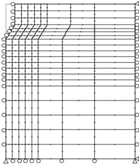
The piezocone penetration was treated as an axi-symmetric boundary problem. The 8-noded isoparametric plane strain element was used. The use of isoparametric elements has an advantage of their capability in describing the curved boundaries in the deformed configuration. A number of trial finite element meshes, resulting in the separation between piezocone and the soil just above the conical tip and in unreasonable negative pore water pressure, were studied with different mesh sizes. The numerical result converges to a unique and reasonable solution with 356.8 mm × 535.2 mm mesh size and four elements along the inclined conical surface. Fig. 3 shows the finite element mesh.

Fig 3 Finite Element Mesh

In the numerical analysis, the total depth of penetration was divided into sub-layers and the steady value of cone tip resistance resulting from the finite element analysis of each layer was obtained, then the

steady value of each layer was smoothly connected to each other as cone tip resistance profile. The same procedure was applied to pore water pressure profile.

This technique was used to avoid tremendous numerical errors resulting from the numerical simulation of the deep and continuous penetration in one step, and successfully worked in this study but more accurate simulation corresponding to real penetration situation needs further research.

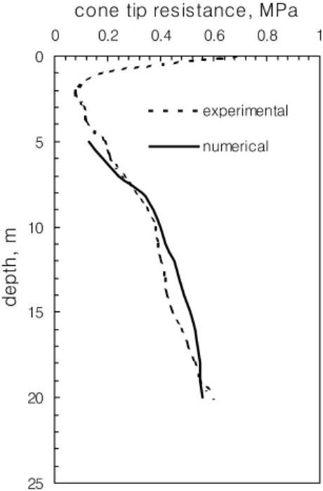
Figs. 4, 5, and 6 show the results of the finite element analysis and the experimental results of the piezocone penetration and dissipation tests conducted in Yangsan site. In Figs. 4 and 5, the numerical results were presented below 5 m depth since the top crust layer was excluded in the numerical simulation. The peak region like in Fig. 4 generally appears to initiate penetration even without the top crust. Fig. 7 indicates the variation of OCR with depth and Figs. 8 to 10 represents the contours of octahedral shear stress, octahedral shear strain, and excess pore water pressure.

0

5

10

15

20

25

0 0.2 0.4 0.6 0.8 1

cone tip resistance, MPa

depth, m

experimental numerical

Fig 4 Cone tip resistance profile

0

5

10

15

20

25

0 0.1 0.2 0.3 0.4 0.5

pore water pressure, MPa

de pth, m

experimental numerical

0.2 0.25 0.3 0.35 0.4 0.45

0 100 200 300 400

time, min.

pore water pressure, MPa

experimental

numerical

O C R 0 0 .5

1 1 .5 2 0

4

8

1 2

1 6

2 0

de pt h, m

Fig 7 Variation of OCR (Kim, D H et al , 1999)

Fig 6 Dissipation curve at 19 m depth Fig 5 Pore water pressure profile

-6 -5 -4 -3 -2 -1 0 1 2 3

0 1 2 3 4 5

normaliz ed radial dis tanc e,r/ro

norm a liz ed v e rti c al di s tanc e,z /ro

10 60

10 10

20

20 20

40 40

Max . Stres s =141 k Pa

Fig 8 Octahedral Shear Stress Contour

-6 -5 -4 -3 -2 -1 0 1 2 3

0 1 2 3 4 5

normaliz ed radial dis tanc e,r/ro

norm a liz ed v e rti c al di s tanc e,z /ro

10 10 10

20

20 20 40

Max . Strain=128 % 5

5 5

40

Fig 9 Octahedral Shear Strain Contour

-6 -5 -4 -3 -2 -1 0 1 2 3

0 1 2 3 4 5

normaliz ed radial dis tanc e,r/ro

norm a liz ed v e rti c al di s tanc e,z /ro

10 60

10 10

20

20 20

40 40

Max . Ex c es s P.W . P.=151 k Pa

Fig 10 Excess Pore Water Pressure Contour

As shown in Figs. 4, 5, and 6, the numerical results showed good agreement with the experimental data.

One reason is that the clay at the site is quite homogeneous. It has been proven during the trimming of samples. The other reason is the use of the Modified Cam-Clay model and the theory of mixtures.

Theory of mixtures successfully simulated especially the dissipation behavior of the clay in the site as shown in Fig. 6. It is well known that the Modifed Cam-Clay model usually gives good prediction for normally consolidated clays. The OCR (overconsolidation ratio) of the site, as shown in Fig. 7, appeared near unity in all depth and even less than unity for the depth below 12 m, which corresponds to the result of the research by Tananka et al. (1999). This can be explained by the fact that the clay is underconsolidated maybe due to the sudden rise of sea level following the Ice Age, or the fact that there are two distinct layers of the clays at the site, where although the mineralogy is the same, the microstructure varies, namely, the upper layer contains large aggregates with bridges in between, while the lower layer is composed of mostly single particles with little aggregation, and much less bridging (Locat and Tananka, 1999). This maybe the reason that the numerical results using the Modified Cam-Clay model, as shown in Fig. 4, showed little better-match with the experimental results in the upper layer since the microstructure in the upper layer shows more clayey characteristics.

In Fig. 5, the numerical results are a little bit larger than the experimental data, which maybe the sluggish behavior of pore water pressure due to incomplete saturation and/or clogging of the filter element.

When penetration stops for dissipation test in heavily overconsolidated clay, it is possible for negative excess pore water pressure measured behind cone tip (u2 type) to occur at the initial part of excess pore water pressure profile (Abu-Farsakh et al., 1997; Kim and Lee, 2000b) but no negative values were measured experimentally and calculated numerically in this study, which is because the soil is not under heavily

overconsolidated. For overconsolidated clay, it is also possible for pore water pressure measured behind cone tip (u2 type) to initially increase before dissipation (Kim and Lee, 2000a). In Fig. 6, no obvious initial increase of pore water pressure was recorded, that confirms the clay is not under overconsolidated state.

Actually, when penetration stops, pore water pressure is influenced by many factors such as stress redistribution, stress relaxation, and viscous and dynamic effects (Kurup, 1993). More frequent reading of measurement and dissipation test at various depth, therefore, might have given interesting results, especially for the very initial stage of dissipation.

7. Summary and Conclusions

In this study, the finite element analysis of piezocone penetration and dissipation tests has been performed.

The results from the finite element analysis have been compared with the experimental results of field piezocone penetration and dissipation tests conducted in Yangsan site. The Modified Cam-Clay model was used to simulate the plastic behavior of the clay based

on Abu-Farsakh et al. (1997). All mathematical equations were formulated in the Updated Lagrangian reference frame to reflect the large displacement and finite strain nature of cone penetration. The results of the numerical analysis showed good agreement with the experimental results all in cone tip resistance profile, pore water pressure profile, and dissipation behavior. The use of the Modifed Cam-Clay model, theory of mixtures, and Updated Lagrangian formulation gave this good result. It needs to be noted that the Modifed Cam-Clay model was successfully applied to this site, of which OCR value is near unity.

Acknowledgments

The authors acknowledge Computer Center of Louisiana State University for helping remote computer work available and Dr. Abu-Farsakh of Louisana Transportation Research Center for helpful suggestions.

The authors are also thankful Jong-Min Park, Gil-Soo Kim, Jung-Gue Park, and Dong-Hee Kim for providing the useful experimental data.

(접수일자 : 2001. 6. 13.)

References

1 Abu Farsakh, M Y , Voyiadjis, G Z , and Tumay, M T (1997), “Numerical Analysis of the Miniature Piezocone Penetration Tests (PCPT) in Cohesive Soils”, International Journal for Numerical and Analytical Methods on Geomechanics (In Press)

2 Bathe, K J (1990), “Finite Element Procedures in Engineering Analysis”, Prentice Hall, Inc , New Delhi, India 3 Chen, W F (1975), “Limit Analysis and Soil Plasticity”, Elsevier Scientific Pub , Amsterdam, Netherlands

4 Chen, W F and Mizuno, E (1990), “Nonlinear Analysis in Soil Mechanics: Theory and Implementation”, Elsevier Science Pub , New York, NY

5 Crisfield, M A (1991), “Nonlinear Finite Element Analysis of Solids and Structures”, John Wiley and Sons, Baffin Lane, Chichester, West Sussex, PO19 1UD, England

6 De Borst, R and Vermeer, P A (1984), “Possibilities and Limitations of Finite Element for Limit Analysis”, Geotechnique, Vol 34, No 2, pp 199～210

7 Desai, C S , Zaman, M M Lightner, J G , and Siriwardance, H J (1984), “Thin Layer Element for Interfaces and Joints”, International Journal for Numerical and Analytical Methods in Geomechanics, Vol 8, pp 19～43 8 Goodman, R E , Taylor, R L , and Brekke, T L (1968), “A Model for the Mechanics of Jointed Rock”, Journal

of the Soil Mechanics and Foundation Engineering, ASCE, No SM3, pp 637～659

9 Kim, D H , Lim, H D , Kim, J W , and Lee, W J , “Evaluation of Permeability Characteristics of Kimhae Clay by Laboratory Tests”, Proceedings of the KGS Spring 2000 National Conference, pp 647～654

10 Kim, G S , Lim, H D , and Lee, W J , “The Effects of Sample Disturbance on Undrained Properties of Yangsan Clay”, Proceedings of the KGS Spring 2000 National Conference, pp 639～646

11 Kiousis, P D , Voyiadjis, G Z , and Tumay, M T (1988), “A Large Strain Theory and Its Application in the Analysis of the Cone Penetration Mechanism”, International Journal for Numerical and Analytical Methods in Geomechanics, Vol 12, pp 45～60

12 Kurup, P U (1993), “Calibration Chamber Studies of Miniature Piezocone Penetration Tests Cohesive Soil Specimens”, Ph D Dissertation, Department of Civil and Environmental Engineering, LSU, pp 240

13 Locat, J and Tananka, H (1999), “Microstructure, Mineralogy and Physical Properties: Techniques and Application to the Pusan Clay”, Proceedings of '99 Dredging and Geoenvironmental Conference, pp 51～31

14 Prevost, J H (1980), “Mechanics of Continuous Porous Media”, International Journal of Engineering Science, Vol 18, pp 787～800

15 Sandven, R (1990), “Strength and Deformation Properties of fine grained Soils obtained from Piezocone Tests”, Ph D Dissertation, The Department of Civil Engineering, The Norwegian Institute of Technology

16 Tananka, H , Mishima, O , Tanaka, M , Park, S Z , and Jeoung, G H (1999), “Consolidation Characteristics of Nangton River Clay Deposit”, Proceedings of '99 Dredging and Geoenvironmental Conference, pp 3～11

17 Teh, C I and Houlsby, G T (1991), “An Analytical Study of the Cone Penetration Test in Clay”, Geotechnique, Vol 41, No 1, pp 17～34

18 Van den Berg, P , Teunissen, J A M , and Huetink, J (1994), “Cone Penetration in Layered Media, an ALE Finite Element Formulation”, Proceedings of 8th IACMAG, West Virginia, USA, in "Computer Methods and Advances in Geomechanics', Siriwardane and Zaman (eds), Balkema, Rotterdam, May, pp 1957～1962

19 Voyiadjis, G Z and Kattan, P I (1989), “Eulerian Constitutive Model for Finite Deformation Plasticity with Anisotropic Hardening”, Mechanics of Materials, Vol 7, pp 279～293

20 Zienkiewicz, O Z et al (1970), “Analysis of Nonlinear Problems with Particular Reference to Jointed Rock Systems”, Proceedings of International Conference of Society of Rock Mechanics, Belgrade, Vol 3, pp 501～509