J. Korean Soc. of Marine Engineering (JKOSME) ISSN 2234-8352 (Online)
http://dx.doi.org/10.5916/jkosme.2014.38.10.1287 Original Paper
This is an Open Access article distributed under the terms of the Creative Commons Attribution Non-Commercial License (http://creativecommons.org/licenses/by-nc/3.0), which permits
†Corresponding Author (ORCID: http://orcid.org/0000-0001-6796-8161): Department of Mechanical & Automotive Engineering, Pukyong National University, YongDang-dong, Nam-gu, Busan, 608-739, Korea, E-mail: [email protected], Tel: 051-629-6158
1 Department of Mechanical & Automotive Engineering, Pukyong National University, E-mail: [email protected], Tel: 051-629-6158 2 Department of Mechanical & Automotive Engineering, Pukyong National University, E-mail: [email protected], Tel: 051-629-6158 3 Department of Mechanical & Automotive Engineering, Pukyong National University, E-mail:[email protected], Tel: 051-629-6158 4 Department of Mechanical & Automotive Engineering, Pukyong National University, E-mail: [email protected], Tel: 051-629-6158
Hybrid control of a tricycle wheeled AGV for path following using advanced fuzzy-PID
Thanh-Luan Bui1 ․ Phuc-Thinh Doan2 ․ Duong-Tu Van3 ․ Hak-Kyeong Kim4 ․ Sang-Bong Kim† (Received October 27, 2014; Revised December 22, 2014;Accepted December 30, 2014)
Abstract: This paper is about control of Automated Guided Vehicle for path following using fuzzy logic controller. The Automated Guided Vehicle is a tricycle wheeled mobile robot with three wheels, two fixed passive wheels and one steering driving wheel. First, kinematic and dynamic modeling for Automated Guided Vehicle is presented. Second, a controller that in- tegrates two control loops, kinematic control loop and dynamic control loop, is designed for Automated Guided Vehicle to fol- low an unknown path. The kinematic control loop based on Fuzzy logic framework and the dynamic control loop based on two PID controllers are proposed. Simulation and experimental results are presented to show the effectiveness of the proposed controllers.
Keywords: Automated guide vehicle, Fuzzy logic controller, Path following, Dynamic modeling, Wheel mobile robot
1. Introduction
Automated Guided Vehicle (AGV) is a transportation ve- hicle automatically traveling on unknown path traced in work- ing environment. AGV is most often used to deliver materials around a manufacturing facility or a warehouse. With lots ad- vantages such as reduction in the number of worker, improve- ment of productivity and quality, improvement of working en- vironment and safety, less damage on transporting goods, re- al-time control of material flow and improved management on product, AGV has become more and more popular and useful in modern industrial production.
Control of AGV for path following has received a great of interest to many researchers because of its nonlinear character- istics caused by nonholonomic constraints of the wheels. Most controllers are designed based on nonlinear techniques [1]-[4]
including the backstepping approach, the sliding mode control, the Lyapunov function approach, the dynamic feedback lineari- zation technique, etc.. Designing controllers using these ap- proaches is rather complex. Furthermore, it requires some de- tailed information related to system parameters, working envi- ronment and complete knowledge of the dynamics that are usually infeasible in practical.
To overcome the above problems, Fuzzy controller is a suitable solution. Fuzzy controller doesn’t require accuracy mathematical modeling of the system. Fuzzy logic controller can control the system with various situations of practical fields. Applying a fuzzy controller is simple, rapid and in- expensive because the rules can be linguistically interpreted by a human expert. Over the latest decade, fuzzy logic has been widely used for mobile robot control [5]-[17]. Precup et al. introduced fuzzy control solution for a class of tri- cycle mobile robots [11]. The control system structure con- tained two control loops to control the forward velocity and the direction of the robot. Antonelli et al. proposed a path following approach for mobile robot using fuzzy-logic set of rules which imitated the human driving behavior [12].
Baturone et al. introduced a design of embedded DSP-based fuzzy controllers for autonomous mobile robots [16]. In pre- vious papers addressing path tracking control, the fuzzy controller used very simple rules and was usually single in- put single output controller [11], while a tricycle WMR needs a multi-input multi-output controller because it has two degree of freedom.
Among 5 types of WMR introduced by Campion et al.
[18], a tricycle WMR is most widely used for industrial
AGV [19]-[20]. However, a detailed report about kinematic and dynamic modeling of tricycle WMR has not been re- ported in literature.
From the above reasons, the purpose of this paper is as follows: First, kinematic and dynamic modeling using the well known Lagrange equation of the AGV is presented.
Second, a hybrid controller that integrates two control loops, kinematic control loop and dynamic control loop, is designed for AGV to follow an unknown path. The kine- matic control loop is based on fuzzy logic framework and the dynamic control loop is based on two PID controllers.
For path following, a tracking error vector is defined. The fuzzy controller uses the tracking error vector as its inputs including position error, angle error and derivative of angle error. From the fuzzy output, velocity control vector at the tracking point is achieved. Because the AGV is driven by a steering driving wheel, steering angle and angular velocity of steering wheel should be calculated. Finally, in dynamic control loop, two PID controllers are used to control two DC motors for tracking the desired steering angle and the desired angular velocity of the steering wheel. Simulation and experimental results are presented to show the effec- tiveness of the proposed controllers.
2. System Modeling
This chapter presents the kinematic and dynamic modeling for the proposed AGV system. This AGV model is based on the model for tricycle wheeled mobile robot introduced by Campion et al. [18].
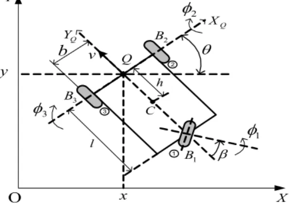
The AGV has two fixed passive wheels and one steering driving wheel. is the radius of two fixed passive wheel and is the radius of the steering driving wheel. Figure 1 shows the coordinate of AGV.
O
XQ
YQ
y Q
x X
Y
q
B2
B3
B1 b v
1 2
3 C
h
l
b
f1
f2
f3
Figure 1: Coordinate for AGV’s modeling
is the global coordinate frame and is the moving coordinate frame. is the tracking point that is placed in the middle of two fixed passive wheels. is the heading angle of AGV.denotes a steering driving wheel.
and denote two fixed passive wheels. axis of moving coordinate frame is passed through the centers of wheels. is the center of mass of the AGV.
is the rotational angle of the wheel. is the steering angle of the steering wheel.
The posture vector of the tracking point on the AGV is specified as follows:
(1)
where are global coordinate of tracking point and is the heading angle of the AGV. Velocity control vector at the tracking point is defined as follows:
(2)
where and are linear velocity and angular velocity at the tracking point .
(3)
The posture vector for total AGV is specified as follows:
(4)
where . Because the AGV is driven by steering driving wheel, kinematic control vector is de- fined as follows:
(5) where denotes
2.1 Kinematic modeling
The contact between the wheels and the ground is supposed to satisfy the pure rolling without slipping condition. This means that the velocity of the contact point is equal to zero and implies that the components of this velocity parallel and orthogonal to the plane of the wheel are equal to zero. With this description, two following constraints are reduced from
three wheels of AGV. Along the wheel plane (pure rolling condition):
(6)
where
cos sin
sin cos
,
cos sin cos
,
Orthogonal to the wheel plane (no slipping condition):
(7)
where
sin cos
It is easy to check that . Therefore, the two last components of Equation (7) are equivalent. Without loss of generality, by removing one of two equivalent con- straints, becomes:
sin cos
The corresponding constraint for no slipping condition Equation (7) is rewritten into:
(8)
From Equation (6) and Equation (8), the following constraint equation is obtained.
(9) where is the × constraint matrix.
The constraint Equation (8) implies that the vector
belongs to the null space of the matrix as follows:
∈ (10)
This is equivalent to the following statement. For all time, there exists a time varying scalar such that the following equation is satisfied:
(11)
where
sin
From Equation (6) and Equation (11), the following equa- tion is obtained.
(12)
where
From Equation (5), Equation (11) and Equation (12), the configuration kinematic model is given as follows:
(13)
where
From Equation (3) and Equation (11), the velocity control vector at the tracking point , is given by:
sin
(14)
From Equation (14), the kinematic control vector can be achieved form as follows:
sin cos
arctan
i f ≠
i f
(15)
2.2 Dynamic Modeling
The potential energy is zero since it is assumed that the AGV is moving on a horizontal plane. The friction energy is ignored. Thus, the total kinetic energy of the AGV is given by [18].
(16)
where ,
,
is the × symmetric matrix with
: mass of the AGV without mass of wheels,
: mass of wheel ,
: distance between the reference point and the center of mass ,
: moment of the AGV without wheels around the verti- cal axis passing through the center of mass of the AGV,
: inertial moment of wheel around the vertical axis passing through ,
: inertia moment of wheel around its axis of rotation,
: distance between the reference point and each wheel,
: the element that lies in the row and the column of matrix ,
where ∼ .
Applying the well known Lagrange equation to the motion of the AGV with nonholonomic constraints, the dynamic equa- tion for the AGV can be obtained as follows [Appendix]:
(17)
where and are scalar functions depending on and .
;
and are the torques applied to the steering wheel for its orientation and rotation, respectively.
Equation (17) can be rewritten as follows:
(18)
where
,
,
and
From Equation (13) and Equation (18), the final system equations are given as follows:
(19)
3. Measurement of Tracking Errors using Camera Sensor
Figure 2 shows schematic for the tracking errors of AGV.
is the position error between the position of the tracking point on the AGV and the reference point on the reference path. is the angle error between the axis and the tan- gent line of the path at the reference point.
Figure 3 shows the schematic of camera window for meas- uring the tracking errors using camera sensor. The camera sen- sor is a Logitech webcam C600. The webcam specification is up to 30 frames per second, 2.0-megapixel sensor and hi-speed USB 2.0 communication. The camera has a resolution of
× .
The camera window is fixed on camera and captures the images of × . The image size is small in compar-
q XQ
YQ
O X
Y
x
y Q
epos
eq
Reference Point
Reference Line
v w
Tracking Point
Figure 2: Schematic for the tracking errors of AGV
epos
Camera window eq
640 pixel
480 pixel (0, 0)
Q ( A, A)
A x y
( C, C) C x y ( B, B) B x y
XQ
YQ
Figure 3: Schematic for measuring the tracking errors using camera sensor
ison with curvature radius of the reference path. Therefore, it is assumed that the image of reference path is straight line as shown in Figure 3.
Form Figure 3, the tracking errors can be obtained as fol- lows:
arctan
(20)
Images captured from web camera are processed by using AForge, NET framework, C# framework designed for developers and researchers in the fields of computer vision and artificial intelligence. To calculate the position error and the angle error from the image captured by camera, image processing procedure includes steps a shown as follows:
Image acquisition
(color image) Color filter Grey image Extract stand alone
objects
Select the object with the maximum size Determine left edge ,
right edge and the center line for the reference line Error
calculation
Figure 4: Image processing procedure
4. Controller Design
To control the AGV for path following, a control algorithm is designed as in Figure 5. The controller integrates two con- trol loops, kinematic control loop based on fuzzy logic frame- work and dynamic control loop based on two conventional PID controllers.
The fuzzy controller uses the tracking error vector as its in- puts including the position error, the angle error and the de-
rivative of angle error. The fuzzy outputs are derivative of the linear velocity, and the angular velocity at the tracking point,.
From the fuzzy output, the velocity control vector at the tracking point is achieved. Because the AGV is driven by the steering driving wheel, the steering angle and the angular ve- locity of the steering wheel should be calculated. Finally, in dynamic control loop, two PID controllers are used to control two DC motors for tracking the desired steering angle and an- gular velocity of the steering wheel.
Reference Path
epos
, e eq&q
w
d,d
h b
1 2
[t t]T
( ), ( ) q t q t&
Dynamic Control Feedback
Kinematic Control Feedback dv
v
Saturation Two PID
Controllers
AGV Dynamic Model Fuzzy
Controller Image acquisition
&
Image processing
òdv
Saturation
Saturation
, h b
[x y ]T
x= q
Eq. (15)
ud
t1
t2 Eq. (19)
Figure 5: Structure of the proposed path-following controller for AGV
4.1 Fuzzy controller Design
Fuzzy rules are normally created based on human experi- ence and logic. Therefore, it is necessary to analyze the de- sired outputs based on available inputs. From two inputs, the position error and the angle error, AGV posture is defined in 9 different situations as shown in Figure 6. From 9 situations, 9 rules are generated, respectively. In addition, two other rules are proposed when derivative of angle error are large, espe- cially while the robot moves away the path with high velocity.
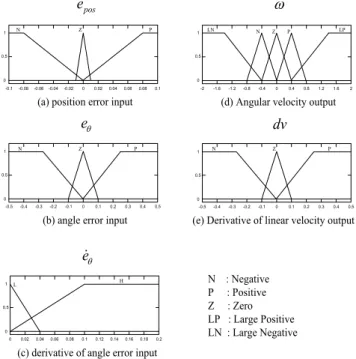
Table 1 shows the fuzzy rules designed for AGV for path following and the membership functions are given in Figure 7.
7
8
9 1
2
3
4
5
6
Reference line
v v v
v v v
v v v
Figure 6: Structure of a fuzzy controller
epos
(a) position error input
eq
(b) angle error input
w
(d) Angular velocity output
dv
(e) Derivative of linear velocity output
N Z P
N Z P
N Z P LP
LN
N Z P
-0.1 -0.08-0.06-0.04 -0.02 0 0.02 0.04 0.06 0.08 0.1 1
0 0.5
1
0 0.5
1
0 0.5 1
0 0.5
-0.5 -0.4 -0.3 -0.2 -0.1 0 0.1 0.2 0.3 0.4 0.5 -0.5 -0.4 -0.3 -0.2 -0.1 0 0.1 0.2 0.3 0.4 0.5
-2 -1.6 -1.2 -0.8 -0.4 0 0.4 0.8 1.2 1.6 2
e&q
(c) derivative of angle error input
L H N : Negative
P : Positive Z : Zero LP : Large Positive LN : Large Negative
1
0 0.5
0 0.02 0.04 0.06 0.08 0.1 0.12 0.14 0.16 0.18 0.2
Figure 7: Membership functions
Table 1: Fuzzy rules
Rules
Inputs Outputs
epos eq e&q w dv
1 N P L N N
2 Z P None N Z
3 P P None Z P
4 N Z None N Z
5 Z Z None Z P
6 P Z None P Z
7 N N None Z P
8 Z N None P Z
9 P N L P N
10 N P H LN N
11 P N H LP N
4.2 PID controller Design
The dynamic control loop includes two PID controllers in Figure 8. The first one is used for tracking the desired steering angle, .
The second one is used for tracking the desired rotation an- gular velocity of steering wheel, .
A PID controller 1 is designed based on steering angle er- ror of the steering wheel as follows:
(21) (22)
where and are the coefficients of the PID con- troller 1.
A PID controller 2 is designed based on rotational angular velocity error as follows:
(23) (24)
where and are the coefficients of the PID con- troller 2.
ò
d dt
1
kp
1
ki
1
kd
d ò h
t2
AGV Dynamic 뭩 Model
t1
b
, , ( )q t h z bd
h
d dt
2
kp
2
ki
2
kd
Figure 8: Dynamic control loop
5. Simulation and Experimental Results
To verify the effectiveness of the proposed controllers, simu- lations and experiments have been done for the AGV to follow an unknown path. In the simulation, the initial values and the numerical parameter values are given in Table 2 and Table 3.
The reference path has five segments with three straight line segments and two curved line segments. The radius of the first curve is 6 m and the radius of the second curve is 4 m.
Figure 9 shows the reference path in simulations and experiments.
The coefficients in two PID controllers are obtained by trial and error method in simulations and experiments. Their nu- merical values are given as follows: , ,
, , , . Figure 10 shows the position error that becomes zero when the path is a
Table 2: Initial values for simulation
Parameters Values Units Parameters Values Units
x0 4 [m] q0 -900 [deg]
y0 1.9 [m] b0 00 [deg]
Table 3: Numerical parameter values of AGV
Parameters Values Units Parameters Values Units
M* 500 [kg] Ip1 10 [kgm2]
m1 10 [kg] Ir1 1 [kgm2]
m2 1 [kg] Ir2 0.05 [kgm2]
m3 1 [kg] Ir3 0.05 [kgm2]
h 0.6 [m] l1 1.22 [m]
rs 0.125 [m] l2 0.268 [m]
rf 0.05 [m] l3 0.268 [m]
I0 250 [kgm2]
(8,8)
(4,2) (8,2)
(14,8) (14,12)
(18,12) (18,16)
(30,16)
X (m) Y (m)
6m
4m
Figure 9: Reference path
0 2 4 6 8 10 12 14 16 18 20
-0.08 -0.06 -0.04 -0.02 0 0.02 0.04 0.06 0.08 0.1 0.12
Time (s)
Position error (m)
simulation experiment
Figure 10: Position error
straight line and is bounded within ± in both simulation and experimental results when the path is a curved line.
Figure 11 shows angle error that is bounded within ± in both simulation and experimental results. Figure 12 shows steering angle of steering wheel in experiment and the steering wheel angle is bounded within ± in both simulation and experimental results. Figure 13 shows the
0 2 4 6 8 10 12 14 16 18 20
-8 -6 -4 -2 0 2 4 6 8
time (s)
angle error (degree)
simulation experiment
Figure 11: Angle error
0 2 4 6 8 10 12 14 16 18 20
50 60 70 80 90 100 110 120 130 140
Time (s)
Steering angle (degree)
Simulation Experiment
Figure 12: Steering angle of steering wheel
0 2 4 6 8 10 12 14 16 18 20
0 0.5 1 1.5 2 2.5
Time (s)
Linear Velocity (m/s)
simulation experiment
Figure 13: Linear velocity of tracking point on AGV
linear velocity of AGV at tracking point
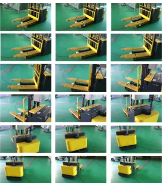
The linear velocity is limited within 0.5m/s and 2m/s in both simulation and experimental results. Figure 14 shows the path following result of the AGV in experiment.
Figure 14: Path following result of the AGV in experiment
6. Conclusions
This paper developed an industrial AGV, a tricycle wheeled mobile robot. First, kinematic model and dynamic model of the AGV were presented. Second, schematic of tracking errors using camera sensor were defined. After that, control algo- rithm for path-following of AGV was proposed based on in- tegration of two control loops, kinematic control loop and dy- namic control loop. The kinematic control loop based on fuzzy logic framework and the dynamic control loop based on two PID controllers were designed. The effectiveness of the pro- posed system was shown through simulation and experimental results. The AGV could follow the desired path with a large enough curvature radius smoothly. So the system could be ap- plied and implemented to the industrial field in practical.
Appendix
Lagrange equation for nonholonomic constraints to the mo- tion of the AGV as follows:
(A.1) The following compact notation is defined.
(A.2)By separating into three components, , and , the following equations are obtained.
(A.3)
(A.4)
(A.5)
where and are the Lagrange multipliers vectors associated with the constrains Equation (6) and Equation (8), respectively.
By eliminating the Lagrange multipliers from Equation (A.3) and Equation (A.5), the following are obtained.
(A.6)
Substituting from Equation (16) to Equation (A.1) can be obtained as the following:
(A.7)
(A.8)
(A.9)
From the kinematic Equation (5), Equation (11) and Equation (12), the following are obtained.
(A.10)
Derivatives of is obtained as follows:
(A.11)
where and are × vectors depending on and .