IEG 환경지질연구정보센터
10
0
0
전체 글
(2) Korean Journal of Remote Sensing, Vol.20, No.3, 2004. 35˚ N. 34.00˚ N. KOREA. 33.50. Jeju. 34 312. 124˚E. 125. 25 30 126. 29.8. 29.7. 29.3. 30.4. ile nm 0 3. 33.00. 205. 204. 30.8. 27.8. Jeju. 22.2. 21.4. 22.4. 25 314 20. 19.6. 21.4. 33. 203. 24.2 25.7 23.1 24.3 22.2 19.0 21.9 21.8 23.7. 313. 32.50 127. 125.00˚E. 128. Fig. 1. Distribution of the measured field surface salinity (psu) around the waters of Jeju Island in August, 1996.. 125.50. 126.00. 127.00. 126.50. Fig. 2-1. Map showing the extended coastal stations for monitoring low salinity water around the Jeju Island in summer season since 1997.. million people. In July and August, floods from torrential MOMAF. rains killed 3.7 million people by drowning, disease and. (Ministry of Maritime Affairs and Fisheries). starvation. The flood affected 51 million people a quarter. NFRDI (National Fisheries Research and Develoment Insitute). of Chinas population at that time (Cox, 2000).. Report. In the summer of 1996, low salinity water less than. Coastal Observing Stations Everyday. 19 psu from the Yangtze River, hit the coastal water around the Jeju Island which is located in the southern. Decision. Cooperation Organizations ·Ministry of Environment ·Research Institute ·Ministry of Government Administration and Home Affairs. Salinity Less than 28 psu. part of the Korean Peninsula (Fig. 1). Marine organisms. Warning. Sea farmer. around the coastal area of the Jeju island were severely. Calling. damaged by low salinity water. The damage was. Operation. Resource Enhancement Institute, Jeju National University, Jeju Provincial Government. amounted to 6 million US dollar by just one occurrence in 1996. After that occurrence, Korean National Fisheries Research and Development Institute (NFRDI). Triangular Observing Network. had to set up the monitoring system on semi-real time. Special Offshore Monitoring Stations. base and the surveys were carried out using research vessels since 1997 (Fig. 2-1, 2-2). However, we need real time monitoring system to detect the distribution of low salinity water around the waters of the Jeju Island.. Every 10 mile Survey. Coastal Monitoring in the Fixed Station Extended Coastal Monitoring Stations Observation per every 3 hours. Fig. 2-2. Observing system for monitoring of low salinity off Jeju Island since 1997.. The salinity itself has no direct colour signal. However, Monahan and Pybus (1978) showed that. Forel scale (Steen and Hoguance, 1990; Hoguance,. yellow substance (the optically active component of. 1997). A negative relationship between salinity and. dissolved organic carbon, DOC) in waters off the West. yellow substance was found in the Kattegat of the Baltic. Coast of Ireland could be related to salinity through the. Sea by Hfjerslev et al. (1996).. colour signal. There were relationships between optical. The aim of this study is to relate the low salinity of. properties of coastal water and salinity observed in. the northern part of East China Sea to the turbid water. fields. Spatial distributions of surface salinity matched. from the Yangtze River using satellite ocean color data. the Secchi depth and the water colour determined using. and transparency instead of Forel scale.. –154–.
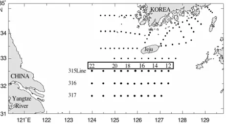
(3) Detection of Low Salinity Water in the Northern East China Sea During Summer using Ocean Color Remote Sensing. 35˚ N. KOREA. 34 Jeju 33 315Line. CHINA. 22. 20. 124. 125. 16. 18. 14. 12. 316. 32. 317. Yangtze River 31 121˚E. 122. 123. 126. 127. 128. 129. Fig. 3. Station map of the NFRDI research cruise.. 2. Materials and methods in situ SS(mg/l). 4.0. The oceanographic data including temperature (˚C), salinity (psu, Practical Salinity Unit), transparency (m) and total suspended solid (mg/l ) were collected in. y=-0.1403x+3.5127 R2=0.51. 2.0 1.0 0.0 0.0. August 1996~2001 on board research vessels of the. (a). n=14 3.0. 5.0. 10.0. 15.0. 20.0. 25.0. in situ Transparency(m). NFRDI in Korea (Fig. 3). The particulate filters were in situ SS(mg/l). weighed to give a measure of suspended solid (SS) in every other observing station. Secchi depths (transparencies) were measured using a standard white Secchi disc at daytime. The data of colour bands from SeaWiFS sensor were received through the antenna located at NFRDI for 4 years (1998~2001).. 8.0 n=16 (b) 7.0 6.0 y=-0.2485x+10.019 5.0 2 R =0.09 4.0 3.0 2.0 1.0 0.0 25.0 26.0 27.0 28.0 29.0 30.0 31.0 32.0 33.0 34.0. in situ Salinity(psu). To relate the satellite ocean color to in situ salinity, we tried to get several empirical relationships between in in situ Salinity(psu). situ SS, transparency and in situ salinity, and between in situ SS, transparency and the ocean color band ratio (490nm/550nm) in normalized water leaving radiances(nLw) from SeaWiFS sensor.. 34.0 n=21 33.0 32.0 31.0 30.0 29.0 28.0 27.0 26.0 25.0 0.0 5.0. (c). y=0.4135x+25.485 R2=0.61. 10.0. 15.0. 20.0. 25.0. in situ Transparency(m). 3. Results First of all, there was relationship between in situ SS and in situ transparency in the East China Sea in 2000. Fig. 4. (a) Relationship between in situ suspended solid (SS) and transparency in the northern part of the East China Sea in August, 2000. Relationship between (b) suspended solid, (c) transparency and salinity.. –155–.
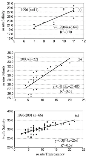
(4) Korean Journal of Remote Sensing, Vol.20, No.3, 2004. Yangtze River Tmin Transparency(m) Tmax. in situ Salinity. Jeju SSY. SSB. 31.0 29.0 27.0 25.0 23.0 21.0 19.0 17.0 15.0. 1996 (n=11). (a). y=1.9204x+6.648 R2=0.70 5. 6. 7. 8. 9. 10. 11. 12. Bottom. in situ Salinity. Fig. 5. Schematic diagram of the vertical distribution of resuspended solid from the shallow bottom and surface suspended solid from the Yangtze River. SSY represents the surface turbid water from the Yangtze River. SSB represents resuspended sediment from seabottom caused by sea wave. Estimated transparency is very high in the waters around Jeju Island than one in the coastal water of the Yangtze River.. 35.0 34.0 33.0 32.0 31.0 30.0 29.0 28.0 27.0 26.0 25.0. (Fig. 4(a)). The relationship between in situ SS and in. 40.0. situ salinity in the East China Sea was not obvious (Fig.. 35.0. 2000 (n=22). y=0.4135x+25.485 R2=0.61 0. 5. in situ Salinity. from the bottom layer in the southern Yellow Sea. Even though most SS come from the bottom, the surface turbid water from the Yangtze River was detected by. we found that good relationships between in situ surface. 25.0 20.0. Sea WiFS(nLw490/nLw555). mentioned below and shown figure 6. Salinity in situ = 1.9024× transparency + 6.648, (n = 11, R2= 0.70) in 1996. Salinity in situ = 0.4135×transparency + 25.485, (n = 22, R2= 0.61) in 2000.. (1996~2001). However it was difficult to find out the match up data between in situ data and SeaWiFS satellite data during. 25. (c). y=0.3844x+26.6 R2=0.58 0. 5. 10. 15. 20. 25. Fig. 6. Relationship between the measured salinity (psu) and the in situ transparency (m) in August (a)1996, (b)2000 and (c)the years (1996∼2001).. the East China Sea in 1996, 2000 and 1996~2001, as. (n = 66, R 2 = 0.58) for 6 years. 20. in situ Transparency. salinity and in situ transparency in the northern part of. Salinity in situ = 0.3844×transparency + 26.600,. 15. 30.0. transparency parameter related to the optical water 4(c) and like the schematic diagram of Fig. 5. Actually,. 10. 1996-2001 (n=66). 4(b)), because most of the total suspended solid come. property from the upper side to the bottom side in Fig.. (b). 6 5. 1998-2001(n=39). 4. y=0.1069x+0.4913 R2=0.32. 3 2 1 0. 0. 5. 10. 15. 20. 25. in situ Transparency(m) Fig. 7. Relationship between the measured field transparency (m) and the band ratio (nLw490/ nLw555) from the SeaWiFS satellite. 39 data sets for transparency were matched between NFRDI’s vessel and SeaWiFS satellite in same spatio-temporal 2 domain within 3 days and 2 km since the last 4 years, 1998~2001.. –156–.
(5) Detection of Low Salinity Water in the Northern East China Sea During Summer using Ocean Color Remote Sensing. in situ Transparency. 25. 2000 (n=19). 15. 33.00. 10. y=8.1698x-2.517. 5. 32.50. 2. R =0.79 0. (a). 33.50˚ N. (a). 20. 0.50. 1.00. 1.50. 2.00. 2.50. 3.00 32.00. SeaWiFS(nLw490/nLw555) 35.0 34.0. in situ Salinity. 33.0. 2000 (n=22). 31.50. (b). 125.00˚E 125.50. 126.00. 126.50. 127.00. 32.0 31.0. (b) SeaWiFS band ratio nLw(490/555nm) 2000. 8. 6 12:22(135E) NFRDI/KOREA. 30.0 29.0. y=0.4135x+25.485 R2=0.61. 28.0 27.0 26.0 25.0 0. 5. 10. 15. 20. 25. Transparency (8.1698*SeaWiFS(nLw490/nLw555)-2.517) Fig. 8. Relationship between (a) the in situ transparency (m), (b) the in situ salinity (psu) and the estimated transparency using the band ratio (nLw490/nLw555) from the SeaWiFS satellite in same spatio-temporal th domain in August 6 , 2000. (a) Match up data sets (19 numbers) between the measured transparency from NFRDI’s vessel and band ratio (nLw 490/nLw 555) from SeaWiFS. (b) Match up data sets(22 numbers) between the measured salinity from NFRDI’s vessel and the estimated transparency related to the SeaWiFS band ratio.. Fig. 9. (a) Distribution of the estimated surface salinity (psu) using the satellite ocean color data with the formula from the relationships between in situ salinity, transparency (m) and (b) SeaWiFS band ratio (nLw490/nLw555) around the waters of Jeju Island in August 6, 2000.. estimated transparency (8.1698×SeaWiFS (nLw490/ nLw555) - 2.517) with the band ratio (nLw490/nLw555). the past. 39 data sets for transparency were matched up. from the SeaWiFS (Fig. 8). When we used only this. between NFRDIs vessel and SeaWiFS satellite in same. relationship (Salinity. spatio-temporal domain within 3 days and 2 km2 since. (nLw490/nLw555)2.517) + 25.485, R2= 0.61) in 2000. the last 4 years (1998~2001) (Fig. 7).. among the other relationships during 1998~2001, we. (psu). = 0.4135(8.1698×SeaWiFS. In case of August 2000, the close relationship. were able to generate the distribution chart of surface. between the in situ transparency and the ratio of. salinity using SeaWiFS data with 1 km spatial resolution. SeaWiFS normalized water leaving radiance (nLw490/. in August 6, 2000 (Fig. 9).. nLw555) was obtained using 19 matched up data for. The distribution of low salinity water in the East. just one year, 2000. Therefore, we were able to set up. China Sea was generated by developing a simple. the simple algorithm related to estimating salinity, using. algorithm in this study in August in 1998, 1999, 2000. the relationship between in situ salinity and the. and 2001 (Fig. 10a′, b′, c′and d′). The result of. –157–.
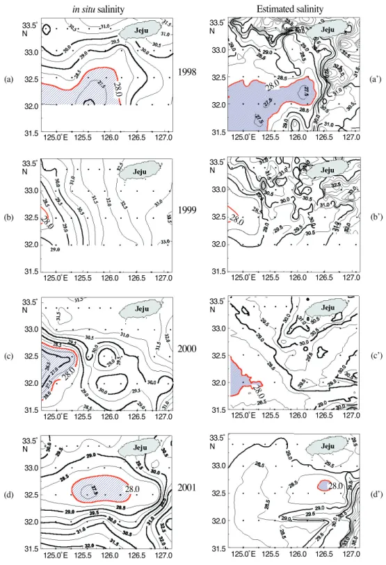
(6) Korean Journal of Remote Sensing, Vol.20, No.3, 2004. Estimated salinity. in situ salinity 33.5˚ N. 33.0. 33.0. 1998. 32.5. 125.0˚E 125.5. 126.0. 126.5. 31.5. 127.0. 33.5˚ N. 33.5˚ N. 33.0. 33.0. 32.5. 1999 .0 28. (b). 126.0. 126.5. 31.5. 127.0. 33.5˚ N. 33.0. 33.0. 2000. 32.5. 127.0. (b’). 125.0˚E 125.5. 32.0. 126.0. 126.5. 31.5. 127.0. 33.5˚ N. 33.0. 33.0. 2001. 28.0. 32.5. 125.0˚E 125.5. 126.0. 126.5. 127.0. (c’). 32.5. 33.5˚ N. 125.0˚E 125.5. 126.0. 126.5. 127.0. 28.0. 32.5. (d’). 32.0. 32.0. 31.5. 126.5. 0 28.. 31.5. 126.0. 32.5 28. 0. 33.5˚ N. 32.0. (d). 125.0˚E 125.5. 28 .0. (c). 125.0˚E 125.5. 32.0. 32.0. 31.5. (a’). 0 28.. 32.0. 32.0. 31.5. 32.5. 28.0. (a). 33.5˚ N. 125.0˚E 125.5. 126.0. 126.5. 31.5. 127.0. 125.0˚E 125.5. 126.0. 126.5. 127.0. Fig. 10. Distribution of surface salinity (psu) in August during 1998-2001. Measured field surface salinity in (a) 68 Aug., 1998, (b) 12-20 Aug., 1999, (c) 4-6 Aug., 2000, (d) 17-23 Aug., 2001. Estimated surface salinity from the SeaWiFS data using the developed regional algorithm in (a’) 4 Aug., 1998, (b’) 19 Aug., 1999, (c’) 6 Aug., 2000, (d’) 16 Aug., 2001.. –158–.
(7) Detection of Low Salinity Water in the Northern East China Sea During Summer using Ocean Color Remote Sensing. 316 Line 22. 21. 20. 19. 18. 17. 16. 15. 14. 13. 12 0 10. 30. 22. 21. 20. 19. 18. 17. 16. 15. 14. 13. Depth(m). 20. 1250 0 10. 30. 22. 21. 20. 19. 18. 17. 16. 15. 14. 13. Depth(m). 20. 50 12 0 10. 30. 22. 21. 20. 19. 18. 17. 16. 15. 14. 13. Depth(m). 20. 50 12 0 10. 30. Depth(m). 20. 50 Fig. 11. Vertical distribution of salinity (psu) at 316 oceanographic observing line in the northern part of the East China Sea.. comparison between the estimated salinity derived from. (Fig. 10b′). However, some parts of the East China Sea. the ocean color satellite and the in situ salinity at the. were covered with clouds. Therefore, SeaWiFS ocean. stations located between Yangtze River and the waters of. color imagery was not good enough to estimate salinity.. Jeju Island, are shown in figure 10. The distribution of. The distribution of 28.00 psu isohaline in the field in. 28.00 psu isohaline in the field around Jeju Island on. 4~6 August, 2000 (Fig. 10c) was similar to the one in. 6~8 August, 1998 (Fig. 10a) was very similar to the one. the estimated salinity on 6th August, 2000 (Fig. 10c′).. the estimated salinity from satellite data on 4th August,. The distributions of 28.00 and 28.50 psu isohalines in the. 1998 (Fig. 10a′). The distribution of 29.00 isohaline in. field in 17~23 August, 2001 were similar to those in the. the field in 12~20 August, 1999 (Fig. 10b) was similar. estimated salinity on 16th August, 2001.. th. to the one the estimated salinity on 19 August, 1999. –159–. The horizontal and vertical distributions of 28 psu.
(8) Korean Journal of Remote Sensing, Vol.20, No.3, 2004. 33.5˚ N. 33.5˚ N. 33.0. 33.0. 32.5. 32.5. 32.0. 32.0. 31.5. 125.0. 125.5. 126.0. 126.5. 31.5. 127.0. 125.0. 125.5. (a) 33.5˚ N. 33.5˚ N. 33.0. 33.0. 32.5. 32.5. 32.0. 32.0. 31.5. 125.0. 125.5. 126.0. 126.0. 126.5. 127.0. 126.5. 127.0. (b). 126.5. 31.5. 127.0. (c). 125.0. 125.5. 126.0. (d). Fig. 12. Horizontal distribution of the differences in salinity (psu) between the measured salinity in field and the estimated one from satellite data in (a) 1998, (b) 1999, (c) 2000 and (d) 2001.. isohaline in the field were wider in 1998 and 2000 than. modern Yellow River. The amount range of surface. those of 1999 and 2001 (Fig. 10, Fig. 11). The. total suspended solid (SS) was 0.6 to 13.30 mg/l. The SS. accuracies were around 0.5~1.0 psu in the western. content of the bottom ranged from 1.28 to 209.44 mg/l. waters of Jeju. However, the highest error ranges. which was the highest SS content value in the water. (1.5~3.0 psu) occurred in some part of the southeastern. column. Obviously, the main reason was resuspension. waters of Jeju, the Kuroshio current region (Fig. 12).. of sediments caused by sea wave (Cai et al., 2001; Lee et al., 2003). However, we were able to detect the main dilution waters from the Yangtze River using the. 4. Conclusions. oceanographic parameter of transparency, which was distinguished from the resuspension of sediments in the. The resource of the terrestrial sediment material in the. seabed.. deep-water area of the southern Yellow Sea was mainly. Our study area, the offshore of the Yangtze River,. originated from the abandoned Yellow River and the. where turbid waters originated from the Yangtze River. –160–.
(9) Detection of Low Salinity Water in the Northern East China Sea During Summer using Ocean Color Remote Sensing. 316 Line 22. 21. 20. 19. 18. 17. 16. 15. 14. 13. 12 0 10. 30. 22. 21. 20. 19. 18. 17. 16. 15. 14. 13. Depth(m). 20. 1250 0 10. 30. 22. 21. 20. 19. 18. 17. 16. 15. 14. 13. Depth(m). 20. 50 12 0 10. 30. 22. 21. 20. 19. 18. 17. 16. 15. 14. 13. Depth(m). 20. 1250 0 10. 30. Depth(m). 20. 50 Fig. 13. Vertical distribution of temperature (˚C) at 316 oceanographic observing line in the northern part of the East China Sea.. meet with the clear Kuroshio warm waters which Secchi. distributions of 28 psu isoline in the in situ field and the. depths is about 25m. These kind of oceanic conditions in. satellite estimated field were wider in 1998 and 2000. the study area make an ideal region for the salinity. than those of 1999 and 2001, is due the presence of very. detection using ocean color. Therefore, the detection of. strong thermocline at about 10 m depth in the western. salinity through an optical signal (the estimated. part of 316 observing station (32 N) in 1998 and 2000. transparency from ocean color satellite) due to yellow. (Fig. 13). We think that the strong thermocline. turbid water from the Yangtze River would be a sensible. prevented low salinity in surface layer water from. approach to monitor the low salinity in the northern part. mixing with high salinity in deep layer water.. of the East China Sea during every summer season.. A simple algorithm, using in the relationships. The reason, why the vertical and horizontal. between the measured salinity, transparency and the. –161–.
(10) Korean Journal of Remote Sensing, Vol.20, No.3, 2004. reflectance ratio of SeaWiFS, shows good agreement. 1999. Semi-analytical moderate-resolution. with the real salinity distribution, which thereby. imaging spectrometer algorithm for chlorophyll. confirms our hypothesis. The developed algorithm will. a and absorption with bio-optical domains based. be useful for early detection and quantification of the. nitrate-depletion temperatures, Journal of. change in surface salinity densities, of the East China. Geophysical Research, 104: 5403-5421.. Sea in summer season.. Chikuni, S., 1985. The fish resources of the northwest Pacific, FAO Fisheries Technical Paper, 266: 67.. Acknowledgements. Cox, J. D., 2000. Ten worst world weather disasters of the 20th century, Weather for dummies. IDG Books, pp. 313-318.. This study was funded by the research project “Operation of application system to produce ocean. Hoguance, A. M., 1997. Shrimp abundance and river. information derived from earth observation satellites” of. runoff in Sofala Bank The rule of Zambezi.. the National Fisheries Research and Development. Paper presented in the workshop on sustainable. Institute and “The application of satellite data for. use of the Cahora Bassa Dam, Songo,. fisheries oceanography” of the Korea Aerospace. Mozambique, 29 September-2 October 1997. Hfjerslev, N. K., N. Holt, and T. Aarup, 1996. Optical. Research Institute.. measurement in the North Sea Baltic Sea transition zone.Ⅰ. On the origin of the deep. References. water in the Kattegat, Continental Shelf Research, 16: 1329-1342.. Bowers, D. G., Harker, G. E. L., Smith, P. S. D., and. Lee, N. K., Y. S. Suh, and Y. S. Kim, 2003. Satellite. Tett, P., 2000. Optical properties of a region of. remote sensing to monitor seasonal horizontal. freshwater influence (The Clyde Sea).. distribution of resuspended sediments in the. Estuarine, Coastal And Shelf Science, 50(5):. East China Sea, J. Korean Associ. Geographic. 717-726.. Information. Studies, 6(3):161-161. (in korean).. Cai D., X. Shi, W. Zhou, and W. Liu, 2001. Sources and. Monahan, E. C. and Pybus, M. J., 1978. Colour, UV. transportation of total suspended matter and. absorbance and salinity of the surface waters off. sediment in the southern Yellow Sea,. the West coast of Ireland. Nature, 274: 782-784. Proceedings of 2nd China-Korea symposium on. Steen, J. E. and A. M. Hoguane, 1990. Oceanographic. sedimentary dynamics and palaeoenviron-. results on expedition carried out by R/V Dr.. mental changes in the Yellow Sea, pp. 9-20.. Fridjof Nansen in Mozambique waters during. Carder, K. L., F. R. Chen, Z. P. Lee, and S. K. Hawes,. –162–. April-May 1990, Relatório, No. 13, 35 p..
(11)
수치

관련 문서
The Dutch physicist Pieter Zeeman showed the spectral lines emitted by atoms in a magnetic field split into multiple energy levels... With no magnetic field to align them,
Modern Physics for Scientists and Engineers International Edition,
Five days later, on 15 January 1975, the Portuguese government signed an agreement with the MPLA, FNLA and UNITA providing for Angola to receive its independence on 11
Usefulness of co-treatment with immunomodulators in patients with inflammatory bowel disease treated with scheduled infliximab maintenance therapy.. Oussalah A, Chevaux JB, Fay
Inclusion and Inclusiveness: Shared Vision of Youth for Local, National, and Global Village Inclusion at large stands for embracing populations with disabilities and
웹 표준을 지원하는 플랫폼에서 큰 수정없이 실행 가능함 패키징을 통해 다양한 기기를 위한 앱을 작성할 수 있음 네이티브 앱과
The index is calculated with the latest 5-year auction data of 400 selected Classic, Modern, and Contemporary Chinese painting artists from major auction houses..
The key issue is whether HTS can be defined as the 6th generation of violent extremism. That is, whether it will first safely settle as a locally embedded group
