농업용 삼륜구동 전기자동차의 후방 속도 및 조향각에 기반한 운동학적 모델
A Kinematic Model Based on the Rear Speed and Steering Angle of Three-Wheeled Agriculture Electric Vehicle
최원식
1
, 프라타마 판두 산디2
, 수페노 데스티아니1
, 변재영1
, 이은숙1
, 양지웅1
, 키프 디마스 하리스 신1
, 전연호3
, 정성원1*
Wonsik Choi 1 , Pandu Sandi Pratama 2 , Destiani Supeno 1 , Jaeyoung Byun 1 , Ensuk Lee 1 , Jiung Yang 1 , Dimas Harris Sean Keefe 1 , Yeonho Jeon 3 , Sungwon Chung 1*
<Abstract>
In this research, tricycle vehicle simulation based on multi-body environment has been introduced. Mathematical model of tricycle vehicle was developed. In this research the left and right wheel speed are calculated based on the rear steering angle and velocity. The kinematic model for the three - wheel drive system was completed and the results were analyzed using the actual vehicle drawings. Through simulink vehicle performance on linear and rotation movement were simulated. Using the mathematical model the control system can be applied directly to the tricycle vehicle. The simulation result shows that the proposed vehicle model is successfully represent the movement characteristics of the real vehicle. This model assists the vehicle developer to create the controller and understand the vehicle during the development process.
Keywords : Agricultural vehicle, kinematic model, tricycle
1* 바이오산업기계공학과, 부산대학교, 교신저자, E-mail: [email protected] 1 바이오산업기계공학과, 부산대학교 2 생명산업융합연구원, 부산대학교 3 근우테크(주)
1 Department of Bio-industrial Machinery Engineering Pusan National University, Korea
2 Life and Industry Convergence Research Institute Pusan National University, Korea
3 Keunwoo Tech Co.Ltd, Daegu, Korea
1. Introduction
Nowadays, research is being conducted on the development of alternative energy and the use of energy in industries. In the automotive sector, environmentally friendly electric vehicles are being commercialized as a solution to alternative energy. In addition, equipment using electric motor instead of conventional combustion engine is being developed in agriculture. Typically, trucks, small-sized working machines, carts and the like are used electric motors. In many other fields, small forklifts used in large marts and factories, electric wagons used in traditional markets, and golf carts for leisure are used similar principles.
The three-wheel drive system is used in agricultural or industrial fields. In this study, a mathematical model based on a kinematical model to simulate a three - wheel drive vehicle were proposed. In vehicle development, it is standard to validate the design results by suitable experiments involving real vehicle. Nevertheless, since experimental setups are usually costly and time demanding, simulation tests are often performed before the real verification [1-6].
This research present the simulation behavior of tricycle vehicle based on MATLAB Simulink.
In this research the tricycle configuration using tadpole configuration that consist of two motorized drive wheel on the front side and one steering wheel on the rear side. The
two front drive wheels are mounted on a common axis, and each wheel can independently being driven either forward or backward.
The aim of our work is to predict the vehicle characteristics and to calculate appropriate velocity of each wheel during normal operation. To do this mathematical model of tricycle was derived and the kinematic model of vehicle is calculated. The vehicle CAD model was developed. Simulation based on MATLAB Simulink using sim mechanics was conducted.
2. Material and Method
Some preparations were needed to make kinematic modeling of the three-wheel-drive train. First, a schematic diagram of the steering angle and specification of the tricycle was obtained. Secondly, mathematical models were obtained according to the boundary condition and kinematic model in driving the tricycle. Finally, we developed a three-wheel drive model of an electric vehicle by referring to the actual specifications used to drive the MATLAB simulation
2.1 Boundary condition of three-wheel drive
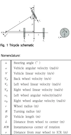
Fig. 1 shows a schematic diagram of
three-wheel drive. In tricycle operation, while
the velocity of each wheel varied for the vehicle to perform rolling motion, the vehicle must rotate about a point that lies along their common left and right wheel axis [7-9].
The point that the vehicle rotates about is known as the Instantaneous Center of Rotation (ICR). Furthermore, the rear wheel also has to be perpendicular to the ICR to avoid skidding condition. Since the motor use two driving wheels on the front side of vehicle, the velocity of each wheel should be calculated precisely to make the vehicle
working properly [10-11].
2.2 Mathematical model
The purpose of forward kinematics in tricycle modeling is to determine vehicle position and orientation based on wheel rotation measurement. By varying the velocities of the two wheels, the trajectories that the vehicle takes can be varied. Since the rate of rotation ω about the ICR must be the same for both wheels, we can write the following equations (1), (2).
(1)
(2)
where is the distance from the center to left and right wheels, , are the right and left wheel linear velocities along the ground, and is the signed distance from the ICR to the midpoint between the wheels.
To avoid skidding of the rear wheel during operation, the moving direction of the rear wheel should be perpendicular to the ICR along
line. The steering angle
can be calculated as follows:
tan
(3)
(4)
The rear wheel velocity then can be calculated as:
V
RV
LICR R
D s
L L
V V
B
LV
Lr
Fig. 1 Tricycle schematic
Steering angle (°)
Vehicle angular velocity (rad/s)
Vehicle linear velocity (m/s)
Back wheel velocity (m/s)
Left wheel linear velocity (rad/s)
Right wheel linear velocity (rad/s)
Left wheel angular velocity(rad/s)
Right wheel angular velocity (rad/s)
Wheel radius (m)
Turning radius (m)
Vehicle length (m)
Distance from wheel to center (m)
Instantaneous center of rotation
Distance from rear wheel to ICR (m) Nomenclature:
(5) where
cos
(6)
Note that a tricycle cannot move in the direction along the axis – this is called constrain. Similar to differential drive vehicles, tricycle are very sensitive to slight changes in velocity in each of left and right wheels.
Small errors in the relative velocities between the wheels can affect the vehicle trajectory.
They are also very sensitive to small variations in the ground plane. At any instance in time we can solve for vehicle linear velocity , angular velocity
and distance to ICR :
(7)
(8)
Combining equation 1 and 8 following equation can be obtained:
(9)
Assume the vehicle is at some position (x, y), headed in a direction making an angle θ with the X axis as shown in Fig. 2. We assume the robot is centered at a point midway along the wheel axle. By manipulating
the control parameters , we can get the vehicle to move to different positions and orientations.
Knowing velocities , and current position of vehicle, using equation 9, we can find the ICR location:
(10)
The following differential equations describe the kinematics of the tricycle:
′
′
′
(11)
Fig. 2 tricycle position
2.3 Kinematic model based on back wheel velocity and steering angle
The input and output were determined to
obtain the kinematic model. Input values are
steering angle (
) and back wheel speed
( ). The output values derived from this are
the left wheel angular velocity (
) and the
right wheel angular velocity (
). The
mathematical value of the three-wheel drive electric train was obtained from the following equations.
Determine the turning radius ( ) based on steering angle (
), Using Eq. 3, the turning radius can be described as follows:
,
(12) Therefore
(13)
Determine the vehicle angular velocity (
) based on back wheel velocity ( ), Using Eq.
5 and 6 the vehicle angular velocity can be calculated as follows:
,
cos (14)
Therefore
cos
(15)
Calculate wheel linear velocities. Linear velocity in the middle of vehicle
Linear velocity on the right wheel:
(16)
Linear velocity on the left wheel:
(17)
Calculate wheel angular velocity using linear velocity based on wheel radius
,
(18)
Replace and
in Eq. 16 and 17 using Eq. 13 and 15, then include in Eq. 18
cos
(19)
cos
(20)
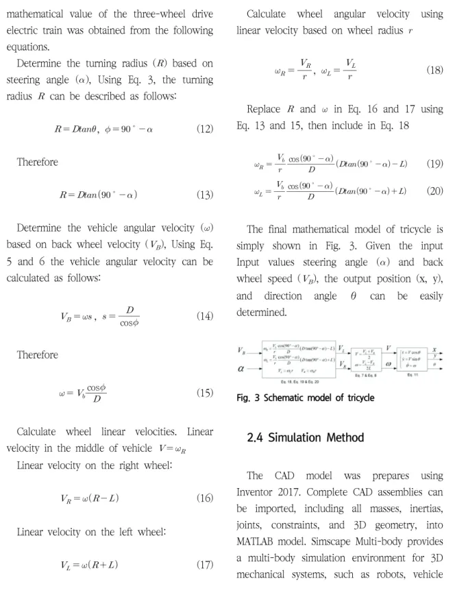
The final mathematical model of tricycle is simply shown in Fig. 3. Given the input Input values steering angle (
) and back wheel speed ( ), the output position (x, y), and direction angle θ can be easily determined.
Fig. 3 Schematic model of tricycle
2.4 Simulation Method
The CAD model was prepares using
Inventor 2017. Complete CAD assemblies can
be imported, including all masses, inertias,
joints, constraints, and 3D geometry, into
MATLAB model. Simscape Multi-body provides
a multi-body simulation environment for 3D
mechanical systems, such as robots, vehicle
suspensions, construction equipment, and aircraft landing gear. You can model multi-body systems using blocks representing bodies, joints, constraints, force elements, and sensors. Simscape Multi-body formulates and solves the equations of motion for the complete mechanical system. The shape of the frame of the used three-wheel drive model is shown in the Fig. 4. The standard size of the wheel is 1240 mm, the width is 574 mm, the diameter of the wheel is 300 mm and the width of the wheel is 95.25 mm.
Fig. 4 Dimension of total assembly
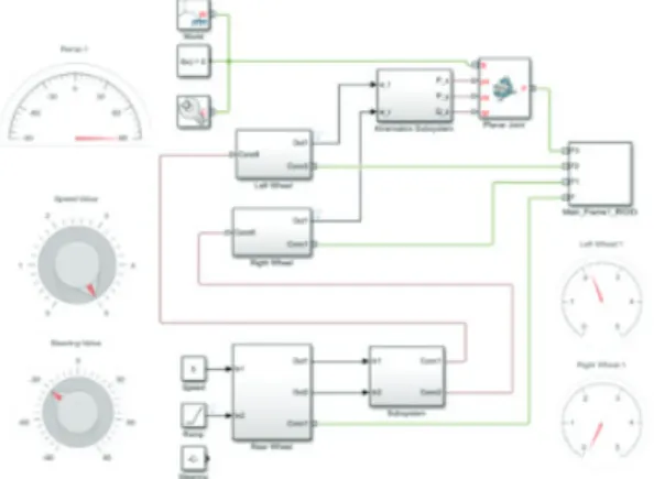
MATLAB Simulink was used and the developed model is shown in Fig. 5. The simulation was performed in two cases. The first simulation was performed by fixing the rear wheel speed and varying the steering angle. The rear wheel speed was changed to 5 km / h and the steering angle was changed from -90 to 90 degrees. D = 1240 mm, L = 287 mm and r = 300 mm. The second simulation was performed by fixing the steering angle and changing the rear
wheel speed. The angle of the steering was fixed at 45 degrees and the speed of the rear wheel was changed from 0 to 5 km / h, which is the same as D = 1240 mm, L = 287 mm and r = 300 mm.
Fig. 5 Simulink simulation of tricyle
3. Result and Discussion
Fig. 6 shows the input for the simulation.
In this example the wheel velocity is
Fig. 6 Steering angle and rear wheel velocity as
input
constant at 5 km/h and the steering angle is varied from -90° to 90°. The simulation time is 9 seconds and the steering angle incremental rate is 20°/s. The purpose of this example is to clarify the relation between steering angle and left and right wheel velocities.
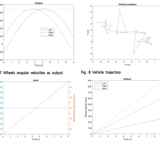
Fig. 7 shows the left wheel, right wheel and back wheel angular velocities as the output. When the steering angle is negative, the right wheel velocity is move faster than the left wheel. When the steering angle is
zero, the left and right wheel is move at the same speed 872.6 rpm. When the steering angle is positive, the left wheel velocity is higher than the right wheel velocity. The rear wheel is move at constant velocity 872.6 rpm during simulation. The maximum velocity is 895.7 rpm.
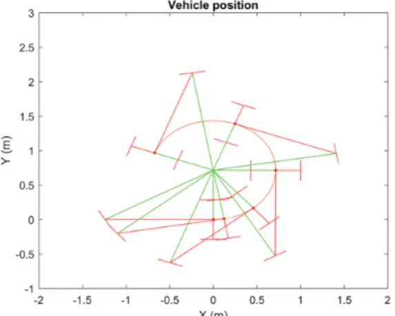
Fig. 8 shows the trajectory obtained from simulation. Green line shows the position of center of rotation R. It shows that the turning radius R is varied according to the steering angle.
Fig. 7 Wheels angular velocities as output
Fig. 8 Vehicle trajectory
Fig. 9 Steering angle and rear wheel velocity as input
Fig. 10 Wheels angular velocities as output
Fig. 9 shows the input for the simulation.
In this example the steering angle is constant at -60° km/h and the velocity is varied from 0 km/h to 5km/h. The simulation time is 9 seconds and the speed incremental rate is 0.555 km/h/s. The purpose of this example is to clarify the relation between rear wheel velocity and left and right wheel velocities.
Fig. 10 shows the left wheel, right wheel and back wheel angular velocities as the output. Since the steering angle is constant, the right wheel velocity, left wheel velocity and back wheel velocity is similar. The wheels velocities is increase gradually proportional to the input back wheel velocity.
Fig. 11 shows the trajectory obtained from simulation. Green line shows the position of center of rotation R. It shows that the turning radius R is constant since the steering angle constant. The back wheel is increase since the velocity is increase.
Fig. 11 Vehicle trajectory
4. Conclusion
MATLAB based simulator for tricycle vehicle has been introduced. Mathematical model of tricycle vehicle was developed. The kinematic model for the three - wheel drive system was completed and the results were analyzed using the actual vehicle drawings.
Through Simulink may simulate vehicle performing linear and rotation movement. At constant wheel velocity 5 km/h and the steering angle is varied from -90° to 90°
simulation, the simulation time is 9 seconds and the steering angle incremental rate is 20°/s, and The maximum velocity is 895.7 rpm. At constant steering angle -60° and the velocity is varied from 0 km/h to 5km/h, the simulation time is 9 seconds and the speed incremental rate is 0.555 km/h/s.
Acknowledgements
This work was supported by Korea
Institute of Planning and Evaluation for
Technology in Food, Agriculture, Forestry
(IPET) through Agriculture, Food and Rural
Affairs Research Center Support Program,
funded by Ministry of Agriculture, Food and
Rural Affairs(MAFRA) (716001-7)
References