Optimal Bankruptcy with a Continuous Debt
Repayment
Byung Hwa Lim*
Department of Economics and Finance, The University of Suwon
(Received: April 6, 2016 / Revised: April 28, 2016 / Accepted: May 23, 2016)
ABSTRACT
We investigate the optimal consumption and investment problem when a working debtor has an option to file for bankruptcy. By applying the duality approach, the closed-form solutions are obtained for the case of CRRA utility function. The optimal bankruptcy time is determined by the first hitting time when the financial wealth hits the wealth threshold derived from the optimal stopping time problem. Moreover, the numerical results show that the investment increases as the wealth approaches the threshold and the value gain from the bankruptcy option is vanished as wealth increases.
Keywords: Debt Repayment, Bankruptcy, CRRA Utility, Consumption, Investment, Duality Approach
* Corresponding Author, E-mail: [email protected]
1. INTRODUCTION
According to the statistics from the Federal Re-serve, each individual including child in United States is over $10.200 in debt and the total outstanding is nearly $3.4 trillion in May 2015. Moreover, due to the high growth rate of consumer debt, the consumer bankruptcy has also sharply increased and about 1% of households in US file for bankruptcy every year by the bankruptcy system. In particular, over 880,000 debtors in US de-clare bankruptcy during 2014. Many countries including South Korea show similar status quo. Thus, it is natural that the study on personal bankruptcy receives much attention. Especially, the determinants and mechanism of consumer bankruptcy are important issues for the policy makers and many researchers are interested in the impacts of bankruptcy on asset pricing, consumption, consumer credit, investment, interest rates, and so on.
The debtors in US can file for bankruptcy from consumer bankruptcy system which consists of Chapter 7 and Chapter 13. By choosing Chapter 7, they receive debt relief and protection from wage garnishment but non-exempt as sets should be paid. So there is no debt after bankruptcy. On the other hand, if the debtors file
for Chapter 13 bankruptcy, the most assets are exempted. Instead, a partial debt remains so they continue to repay the reduced debt. This is similar to the individual reha-bilitation system in South Korea, which is introduced in 2004.
In this paper, we consider an individual’s optimal consumption and investment choice problem when there is a continuous debt repayment and option to file for ban-kruptcy. The model is in line with Chapter 7 of personal bankruptcy system in US. Thus, the debtors receive an exemption from the repayment by filing for bankruptcy in exchange for a partial wealth as a penalty. Unlike Chap-ter 13, they can enjoy the full wage afChap-ter bankruptcy and participate in financial market.
We apply the duality approach to obtain the closed-form solution. Since the option to go bankrupt makes it possible to stop paying the repayment, the debtors might choose bankruptcy if the value of expected utility with punished wealth is larger than the value with a continu-ous debt repayment. Thus, they choose the optimal time to file for bankruptcy, which means that we have to treat the optimal stopping time problem like an optimal re-tirement choice. Accordingly, by comparing the model without the option, it is possible to get the option value.
This paper has two contributions. We first model the optimal bankruptcy problem with labor income and obtain the explicit solution by applying the duality ap-proach. The second one is specific results for consump-tion, investment, bankruptcy time, and option value. Not surprisingly, due to the existence of the option, the op-timal consumption rate and investment are higher than those of the model without the option near bankruptcy wealth boundary. After bankruptcy, the optimal polices are always lower than those of Merton’s problem (Mer-ton, 1971) because of the punishment at bankruptcy. Moreover, the option value decreases with wealth level, which represents the value gain from the option van-ishes as wealth increases.
There are large strand of literature related to per-sonal bankruptcy. Economic models for consumer bank-ruptcy and credit are surveyed in Livshits (2015). Borgo (2015) investigates the impact of bankruptcy protection on investment empirically. Theoretically, Sethi (1998) surveys the portfolio choice problems subject to bank-ruptcy. Typically, the event of bankruptcy in those stud-ies determines an endogenous or exogenous minimum wealth boundary rather than optimal time to bankruptcy. Recently, Choi et al. (2015) provides explicit expres-sions for the minimum wealth boundary when the eco-nomic agent faces market participation constraint. Up to our best knowledge, Jeanblanc et al. (2004) is the clos-est work to ours. However, they apply the dynamic pro-gramming principle (DPP) to the optimal bankruptcy problem with no wage income. So the wealth should always be positive.
This paper is organized as follows. Section 2 de-scribes the financial market with bankruptcy system. The problem with an option to go bankrupt and its explicit solutions are provided in Section 3. Section 4 shows the numerical implications and Section 5 concludes.
2. THE FINANCIAL MARKET
We consider a continuous time financial market with two assets which are a riskless asset and a risky asset. The riskless asset has a risk free rate r (> 0) and the risky asset evolves
, t t t dS dt dB S =μ +σ
where Bt is a standard Brownian motion under the regu-lar probability space ( ,Ω F,P) where F is the filtration generated by the Brownian motion
{
B tt, < ∞}
, The pa-rameters μ andσ are constant coefficients which make the risky asset as a Geometric Brown motion.The infinitely-lived working agent has to pay a fixed rate (d > 0) as a debt repayment until bankruptcy. He receives constant income stream ε forever and the repayment debt is supposed to be independent of credit
borrowing based on labor income. The collateral debt from house might be an example which is independent of credit borrowing. If the fixed debt repayment is large compared to the labor wage, the agent would more likely try to file for bankruptcy even though the finan-cial wealth is not low enough. In our model, it is sup-posed that the agent can choose his bankruptcy time τ with a fixed cost F(> 0) as redemption and a certain portion of remaining wealth should be paid as a penalty.
It is assumed that the decision of bankruptcy is ir-reversible and there is no difference between the income streams before and after that event. In addition, the agent can continue to consume and participate in the financial market even after bankruptcy. In reality, in the case of bankruptcy, it is impossible to invest in the risky assets or borrowing from financial institutions for a while. Then there would be a chance to relief from bankruptcy so that he can participate in the financial market again.
Let’s denote the consumption rate and portfolio as
t
c and πt.The consumption rate is supposed to be Ft
-adapted nonnegative process with
0 , , . .
t s
c ds< ∞ ∀ < ∞t a s
∫
and the portfolio amount is also Ft-adapted measurable
process with 2
0 , , . .
t
sds t a s
π < ∞ ∀ < ∞
∫
Then the wealthdy-namics, X Xt( 0=x), is unfolded by ( ( ) ) , ( ( ) ) , t t t t t t t t t t t rX r c d dt dB t dX rX r c dt dB t π μ ε σπ τ π μ ε σπ τ + − − − + + ≤ ⎧ = ⎨ + − − + + ≥ ⎩ (1)
Notice that the agent does not need to pay a fixed rate d anymore after bankruptcy. Moreover, he keeps receiving same income stream with that before bankruptcy. Not to default at the initial time, the initial wealth is supposed to be greater than (−ε/r+ +F η), whereη is a small required amount he has to consume. The lower bound of initial wealth consists of three components. The first one is a remaining human capital or credit bor-rowing from the future income. The second term, F, makes it possible for the agent to declare his bankruptcy voluntarily and the last term can be thought of a mini-mum consumption after default. Thus, the natural liquid-ity constraint is derived by
t
X F , t 0.
r
ε η
≥ − + + ≥
If we define the pricing kernel and market price of risk by Ht e rtZt
−
≡ and θ≡(μ−r) /σ where Zt=exp
2 0 2 0 t t s ds dB θ θ ⎛ ⎞ − + ⎜ ⎟ ⎜ ⎟
⎝
∫
∫
⎠ is an exponential martingale, thedynamic wealth process before bankruptcy in (1) can be transformed into the following static budget constraint as 0 0H ct(t d )dt H X x, S0, τ τ τ ε τ ⎡ + − + ⎤≤ ∈ ⎢ ⎥ ⎣
∫
⎦ E (2)where E0[ ]⋅ is a conditional expectation at time 0 and 0
S is a set of optimal stopping time which is F-mea-surable.
3. THE OPTIMIZATION PROBLEM
The infinitely-lived working agent wants to maxi-mize his expected utility and has an option to file for bankruptcy. If he goes bankrup, he has to pay a fixed cost F and a certain portfolio of remaining wealth should be paid as a penalty. Instead, the labor income is pre-served so the strategic trading is possible with it. It means after bankruptcy, the agent behaves optimally without any constraints except for the reduced wealth. Thus, the objective function is expressed as follows.
0 , , V(x) max ( ) t t t c u c dt π τ ∞ ⎡ ⎤ = ⎢ ⎥ ⎣
∫
⎦ E 0 , , max ( ) ( ( )) , t t t t c e u c dt e V X F τ β βτ τ π τ α − − ⎡ ⎤ = ⎢ + − ⎥ ⎣∫
⎦ E %where the function V%( )⋅ is a value function after bank-ruptcy. Note that the bankrupt time is a stopping time τ determined endogenously. Since the agent has to pay a bankruptcy cost and penalty at τ, the value function should be a function of the remaining. If we denote the time right after default asτ+, the last term of the objec-tive function is a value function of Xτ ,
+ which isV%
(
)
(Xτ ) V α(Xτ F) ,
+ = % − where α is a positive constant
which is less than one.
For the model tractability and closed expressions, we consider CRRA utility function defined by
1 t 1 , 1, 0, 1 u(c ) log , 1, t t c c γ γ γ γ γ − ⎧ ≠ > ⎪ − = ⎨ ⎪ = ⎩
Throughout this paper, we assume γ≠0 and γ>0 with-out any information loss. Then the value function after default becomes 1 1 ( ) , (1 ) t t V X X r K γ γ ε γ − ⎛ ⎞ = ⎜ + ⎟ − ⎝ ⎠ %
where the constant K is a constant defined by K≡ +r
2 2 1 . 2 r β γ θ γ γ − + −
Notice that the value functionV X%( t) is the same value function with the classical Merton’s problem (1971) when the agent receives a constant in-come ε. In sum, our objective function is rewritten as follows.
Problem 3.1: The economic agent wants to maximize
his expected utility function by choosing consumption
rate, investment, and bankruptcy time. i.e., the value function is given by 1 0 , , 1 ( ) max 1 t t t t c V x τe β c γdt π τ γ − − ⎡ = ⎢ − ⎣
∫
E 1 1 ( ) , (1 ) e X F r K γ βτ τ γ ε α γ − − ⎛ ⎞ ⎥⎤ + ⎜ − + ⎟ − ⎝ ⎠ ⎦⎥subject to the static budget constraint (2).
Notice that Problem 3.1 does not contain the natu-ral borrowing limit, −ε/r+ +F η. This is because the agent could never reach that boundary by choosing the bankruptcy. In the other words, the wealth threshold of bankruptcy is higher than the natural borrowing limit so that liquidity constraint never binds.
We apply the duality approach to resolve Problem 3.1. Jeanblanc et al. (2004) consider the similar problem but they do not consider the labor income even before bankruptcy. Moreover, they apply the DPP developed in Karatzas et al. (1987). Thus, our method has more ad-vantage in proving the optimality of solution.
By introducing a Lagrange multiplier λ( 0),> let’s define the dual value function as
1 0 , , 1 ( ) max 1 t t t t c v x τe β c γdt π τ γ − − ⎡ = ⎢ − ⎣
∫
E 1 1 ( ) , (1 ) e X F r K γ βτ τ γ ε α γ − − ⎛ ⎞ ⎥⎤ + ⎜ − + ⎟ − ⎝ ⎠ ⎦⎥ 0H ct(t d )dt H X . τ τ τ λ ⎡ ε ⎤ − ⎢ + − + ⎥ ⎣∫
⎦ E (3)It is well-known that the dual value function is re-duced to an optimal stopping time by maximizing over the consumption and financial wealth at bankruptcy. Mo-reover, the derived optimal stopping time problem should satisfy a certain variational inequality. This approach is widely used for solving the optimal retirement problem. The disutility before retirement, higher leisure, and grea-ter utility afgrea-ter retirement are typical examples for in-centives to retire. Our optimal bankruptcy problem also has an incentive to go bankrupt. The agent would file for bankruptcy if he might think the continuous debt repay-ment is too painful. After bankruptcy, he is relieved from the debt payment with fixed cost and penalty. So the bankruptcy happens when the value of the status with continuous debt repayment and the value of the status with no debt repayment in exchange for reduced wealth match.
Let’s define an auxiliary function φ( , )t y as 1 1 ( ) ( , ) sup ( ) 1 t y y s t s s t t y τe β y γ d y ds τ γ φ ε γ − = ⎡⎢ − − ⎛⎜ ⎞⎟ ≡ ⎢ − − ⎜ − ⎟ ⎝ ⎠ ⎣
∫
E1 1 ( ) , (1 ) s t y e R y K r γ β τ τ γ ε γ α α − − − ⎤ ⎛ ⎞ ⎛ ⎞ ⎛ ⎞ ⎥ ⎜ ⎟ + ⎜ ⎜ ⎟ +⎜ − ⎟ ⎟⎥ − ⎝ ⎠ ⎝ ⎠ ⎜ ⎟⎥ ⎝ ⎠⎦
where the dual variable yt(=λe Hβt t) has its dynamics as
(
)
t dy . t t r dt dB y = β− −θFor a given differential operator L,
2 2 2 2 1 ( ) , t β r y y 2θ y y ∂ ∂ ∂ = + − + ∂ ∂ ∂ L
the function φ( , )t y can be obtained from solving the optimal stopping time problem which satisfy the follow-ing variational inequality:
Variational Inequality 3.1
Find the free boundary y which indicates the wealth level at bankruptcy and a function φ( , )t y ∈C (0,1
(
∞ ×)
(
)
(
{ }
)
2 ) C (0, \ y + ∩ ∞ × + R R satisfying 1) 1 1 ( , ) ( ) 0, 1 t t y e β γ y γ d y φ ε γ − − ⎧⎪ ⎫⎪ + ⎨ − + − ⎬= ⎪ ⎪ ⎩ ⎭ L 0< ≤y y, 2) 1 1 ( , ) ( ) 0, 1 t t y e β γ y γ d y φ ε γ − − ⎧⎪ ⎫⎪ + ⎨ − + − ⎬≤ ⎪ ⎪ ⎩ ⎭ L , y>y 3) 1 ( , ) , (1 ) t y t y e F y K r γ γ β γ ε φ γ α α − − − ⎛⎜ ⎛ ⎞ ⎛ ⎞ ⎞⎟ > ⎜ ⎜ ⎟ +⎜ − ⎟ ⎟ − ⎝ ⎠ ⎝ ⎠ ⎜ ⎟ ⎝ ⎠ 0< ≤y y, 4) 1 ( , ) , (1 ) t y t y e F y K r γ γ β γ ε φ γ α α − − − ⎛⎜ ⎛ ⎞ ⎛ ⎞ ⎞⎟ > ⎜ ⎜ ⎟ +⎜ − ⎟ ⎟ − ⎝ ⎠ ⎝ ⎠ ⎜ ⎟ ⎝ ⎠ y>y for all t > 0.Since φ(0, )λ =v( )λ by definition, it is suffice to solve the optimal stopping time problem to get the value function. Let’s denote the positive real root of the fol-lowing quadratic equation by n+( 1),>
2 2 2 1 1 0. 2θ n β r 2θ n β ⎛ ⎞ +⎜ − − ⎟ − = ⎝ ⎠
Then, the next proposition provides the answer to Variational Inequality 3.1 and thus, the dual value func-tion (3).
Proposition 3.1 The dual value function v y( ) in (3) is determined by 1 1 1 1 , 0 , (1 ) ( ) , , (1 ) n d Cy y r y y K r v y y F y y y K ar γ γ γ ε γ γ ε γ α + − − ⎧ − ⎪ + + < ≤ ⎪ − ⎪ = ⎨ ⎪ ⎛ ⎞ ⎛ ⎞ ⎪ ⎜ ⎟ +⎜ − ⎟ > − ⎪ ⎝ ⎠ ⎝ ⎠ ⎩
where the free boundary y and the coefficient C are determined by
(
)
1 1 ( 1)( 1) 1 , 1 1 d K n F r r y n γ γ γ ε γ α γ γ α − + − + ⎛ ⎞ ⎜ − − ⎛ ⎛ − ⎞− + ⎞⎟ ⎜ ⎜ ⎜⎝ ⎟⎠ ⎟⎟ ⎝ ⎠ ⎜ ⎟ = ⎜ ⎛ ⎞ ⎟ ⎜ + − ⎜ − ⎟ ⎟ ⎜ ⎜ ⎟ ⎟ ⎜ ⎝ ⎠ ⎟ ⎝ ⎠ and 1 1 1 1 1 n C y Kn γ γ γ α + − − + − + ⎛ ⎞ ⎜ ⎟ = − ⎜ ⎟ ⎝ ⎠ 1 1 1 1 d F y n . n r r ε α −+ + ⎛ ⎛ ⎞ ⎞ − ⎜ ⎜ − ⎟− + ⎟ ⎝ ⎠ ⎝ ⎠Proof: For 0< ≤y y, if we suppose the solution to Vari-ational Inequality 3.1 is separable as φ( , )t y =e−βtϕ( ),y
the function ϕ( )y satisfies the following ordinary dif-ferential equation (ODE),
1 1 2 2 1 ( ) ( ) ( ) ( ) 2 y y r y y y 1 y γ γ θ ϕ β ϕ βϕ γ − ′′ + − ′ − + − (ε d y) 0. + − =
Since the particular solution of above ODE is given by 1 1 ( ) , (1 ) p d y y y K r γ γ ε ϕ γ − − = +
− the general solution should
have the form of
1 1 1 2 ( ) , 1 n n d y C y C y y y r γ γ ε ϕ γ + − − − = + + + −
where C1 and C2 are constant coefficients and the
pow-ers n ( 0)+ > and n ( 0)− < are two roots of the quadratic
equation derived from the homogenous equation. How-ever, this function is ill-posed y=0 if the coefficient
2
C is nonzero. Thus, C2 should be zero by the growth condition.
boun-dary value are determined by the value-matching and smooth pasting conditions at the free boundary. ■
It is easy to check that the free boundary value y is well-defined since d r/ should be larger than F. How-ever, the sign of the coefficient C is uncertain and it depends on the market parameters.
Now we can state our main result which gives the analytic expressions of the optimal policies including optimal bankruptcy time.
Theorem 3.1 The value function in Problem 3.1 is
ob-tained from
{
}
0 ( ) ( ) , V x min v x λ> λ λ = +where the dual value function v y( ) is given in Proposi-tion 3.1.
Furthermore, the optimal wealth process, consum-ption rate, and investment before bankruptcy are deter-mined respectively by 1 * * 1 * n 1 , t t t d X Cn y y K r γ ε +− − + − = − + − * 1 * * , n t t t d c K X CKn y r ε +− + − ⎛ ⎞ = ⎜ + ⎟+ ⎝ ⎠ * 1 * * 1 1 n , t t t d X Cn n y r θ ε θ π γ σ σ + γ + +− ⎛ ⎞ − ⎛ ⎞ = ⎜⎝ + ⎟⎠+ ⎜ + − ⎟ ⎝ ⎠
where the dual variable y*t *e Ht t β λ = satisfies 1 * * 1 1 0. n e Cn x K r γ ε λ +− λ− + − + − + =
Furthermore, the optimal time to bankrupt is de-fined by the first hitting time as
{
}
* 0 * ,
t
inf t X x
τ = ≥ ≤
where the bankruptcy wealth level x is determined by
1 1 1 . n d x Cn y y K r γ ε +− − + − = − + −
Proof: It is not trivial that the value function can be
ob-tained from choosing minimum Lagrange multiplier. This is because to get the original value function in Problem 3.1 by applying duality approach, the minimization pro-blem over λ and the optimal stopping time problem should be considered simultaneously. In Karatzas and Wang (2000), however, it is well-documented that any orders between two problems have the same values. Thus, the minimization problem with dual value
func-tion v y( ) which is the solution to the optimal stopping time problem provides the original value function.
The first order condition with respect to λ be-comes v y′( *)+ =x 0. Thus, if we substitute dual variable
*
t
y whose initial value is λ*into the first order condi-tion, the optimal wealth process is derived. In particular, we have
( )
* *
t
X = −v yt
Moreover, the optimal consumption rate is determined when the original problem is transformed into the dual value function v y( ). By using the dual variable *,
t y the optimal consumption rate is given by
1 * * t c yt γ, − =
The optimal investment in risky asset is actually the volatility of the wealth process. Therefore, if we apply Ito’s formula to the optimal wealth process, the coeffi-cient of diffusion term determines the investment amount. Finally, the optimal bankruptcy is directly related to the optimal hitting time of dual variable y*t defined by
{
}
* 0 * . t inf t y y τ = ≥ ≥From the same spirit from Lemma 8.1 of Karatzas and Wang (2000), the dual value function v y( ) is strictly de-creasing and strictly convex, which guarantees the one-to-one correspondence between the dual variable and the wealth level. The optimal stopping time, therefore, can be converted to the expression using the bankruptcy wealth boundary x. ■
The analytic expression helps to understand the ef-fect of the existence of bankruptcy option. In particular, the optimal time to go bankrupt is determined by the first hitting time to reach the critical wealth level x.
That implies that the agent never bankrupts if the wealth level is higher than the threshold.
When there is no such anoption without any debt repayment, the optimal consumption and investment are given by * , * . ben ben t t t t c K X X r r ε π θ ε γ σ ⎛ ⎞ ⎛ ⎞ = ⎜ + ⎟ = ⎜ + ⎟ ⎝ ⎠ ⎝ ⎠
Thus, our model has two differences compared to the benchmark. The human capital at the beginning is reduced to (ε−d) / ,r which implies that the agent could borrow against his future income except the current value of debt repayment. The additional terms of the optimal policies represent the effect of the existence of
bankruptcy option. Since the sign of the constant C de-pends on the market parameter, the impact is uncertain but it determines the impact of bankrupt option we are interested in positive C. To figure out the value of the option, we need to compare our optimal values with the problem with debt payment and without default option. Thus, the consumption rate and investment of the other benchmark would be 2 * 2 * , . ben ben t t t t d d c K X X r r ε π θ ε γ σ − − ⎛ ⎞ ⎛ ⎞ = ⎜ + ⎟ = ⎜ + ⎟ ⎝ ⎠ ⎝ ⎠
In the next section, for given market parameters we show the numerical results which describe the optimal behaviors near the critical wealth boundary in more de-tails.
4. IMPLICATIONS
The numerical results of the optimal consumption rate and investment are illustrated. We adapt the market parameters from Dybvig and Liu (2010), which are
0.07, 0.18,r 0.01, 0.07, 2, 0.4
μ= σ= = β= γ= ε=
Moreover, the continuous debt repayment, a fixed cost at bankruptcy, and the penalty constant are sup-posed to have
0.1, / 0.5, 0.7.
d= F=d r× α=
The given parameters represent that the agent can choose his bankruptcy by paying a half of remaining total debt ( / )d r and 30% of his remaining wealth after debt payment as a penalty (0.3 (× x−0.5 ( / )).× d r Thus, after default the agent can keep 70% of total remaining wealth and behaves optimally with that wealth as an initial wealth. At this stage, there is no debt repayment and receives the same labor income with that before de-fault.
As mentioned, we introduce two benchmark mod-els to investigate the effect of bankruptcy option. The model without debt repayment and the option (B1) is the first benchmark and the model without the option is the second one (B2). Since the difference between two mo-dels is the continuous debt repayment, it is clear that the slope of optimal consumption rate and investment are equal. Instead, the human capital or credit borrowing is reduced by the amount of total debt repayment (d/r).
For given market parameters, the natural wealth limits of B1 and B2 are -40 and -30 respectively. More-over, the critical wealth level is given by -0.73. Notice that even though the labor income is higher than the debt repayment, the agent chooses his bankruptcy. This is because he wants to enjoy his full income without any loss. In addition, the bankruptcy threshold can be
posi-tive. For instance, if we assume the continuous debt repayment as 0.15, the threshold increases to 7.57.
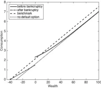
Figure 1 shows the optimal consumption rate corre-sponds to the financial wealth. Before bankruptcy, the consumption level of our model is higher than that of B2.The difference can be considered as the value of bankruptcy option. Intuitively, the option premium would be larger as the wealth approaches the threshold and Figure 1 describes this fact. As a result, the marginal pro-pensity to consume (MPC) becomes smaller near bank-ruptcy boundary and this never happens if there is no such an option. On the other hand, as wealth increases, the consumption of our model approaches that of B2. This is because the value of the option to default van-ishes if wealth level is high enough. At the bankruptcy, due to the repayment and a penalty there is a large drop. After bankruptcy, the consumption rate is always less than that of B1 and the natural minimum boundaries coincide.
Figure 1. Optimal Consumption Rate
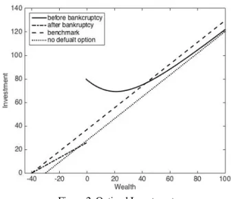
Figure 2 illustrates the optimal investment in the risky asset corresponding to the wealth level. Similar to the consumption rate, there is a big jump at the critical wealth boundary. Furthermore, the investment before bankruptcy is larger than that of B1 and it is less than that of B2 after bankruptcy. Surprisingly, there is a wealth level which provides the minimum investment. This implies the investment level increases as the wealth level approaches the threshold for bankruptcy. In words, the agent invests more even if his wealth level is lower than the wealth at minimum investment. The intuition is as follows. When the agent’s wealth level approaches the critical boundary, he takes more risk to make the wealth higher. This is possible because if there is a posi-tive market shock the higher investment helps to escape from being on the verge of bankruptcy as soon as possi-ble. If the market has a bad shock, however, he would file for bankruptcy by giving up some portion of remain-ing wealth after redemption as a punishment. We want
to point out that this scenario could happen only when the agent has an option to go bankrupt.
Figure 2. Optimal Investment
In Figure 3, we describe the option value depend-ing on the wealth. For a fixed wealth level, the option value is defined by the difference between the value functions with and without the default option. Since the consumption rate and investment approach to those of B2, we can expect decreasing option value in wealth. As a result, near threshold (x= −0.73), the ratio of option premium is about 22% but that ratio decreases to 10% if the wealth is near 20.
Figure 3. Option Value. The Option Value for a Fixed Wealth Level is Defined by the Difference be-tween the Value Functions with and Without the Default Option
To focus more on the bankruptcy boundary, we provide the comparative static results in Table 1. The natural borrowing limit without any debt repayment is 40 since the wage income is fixed as 0.4. According to the given parameters, the critical wealth can be both
positive and negative. The agent with larger risk aver-sion declares his default with higher wealth level. This implies that if his initial state stays before bankruptcy, a more risk-averse agent chooses his default earlier. Fur-thermore, if the penalty becomes severe, which means the agent has to pay a higher percentage of remaining wealth right after his repayment F, the bankruptcy thresholds are sharply dropped. This is because the value function after default is too low due to the low initial wealth. We can explain the effect of predeter-mined repayment F similarly.
Table 1. Comparative Static Results of x. The Parameter Values of α α1, 2, F1, F2, F3, d1, d2, and d3 are given by α1=0.7, α2=0.5, F1=d r/ ×0.2, F2= 3 1 2 / 0.3, / 0.4, 0.1, 0.15, d r× F =d r× d = d = and 3 0.2 d = 2 γ= γ=3 x 1 d d2 d3 d1 d2 d3 1 F 3.2 13.5 23.8 10.2 21.6 33.0 2 F 1.9 11.5 21.2 8.6 19.2 29.8 1 α 3 F 0.6 9.6 18.5 7.0 16.8 26.6 1 F -15.8 -9.7 -3.5 -6.7 0.3 7.2 2 F -16.1 -10.1 -4.1 -7.2 -0.5 6.3 2 α 3 F -16.4 -10.6 -4.6 -7.6 -1.2 5.3 The impact of continuous debt repayment on the threshold is worth to highlight. Our comparative static result tells that the larger debt payment the agent has to pay before bankruptcy, the higher critical wealth level he chooses for bankruptcy. In particular, when d=0.2,
then a half of wage income (ε=0.4) should be paid for the debt. Thus, the agent suffers too much and has more incentive to stop paying the debt. Moreover, since there is no loss on the labor income after bankruptcy, his value function after default becomes relatively higher. So if the bankruptcy is inevitable, he tries to go bankrupt as soon as possible.
5. CONCLUSIONS
We investigate the optimal bankruptcy time when the agent has a continuous debt repayment and receives a labor income. By applying the duality approach, the closed-form solutions are provided. Especially, the op-timal time to file for bankruptcy is determined by the first hitting time when the wealth level reaches a certain threshold. Numerical results show that the bankruptcy option premium increases as the wealth approaches to that threshold and it leads to higher consumption rate and investment compared to the problem without such an option. Surprisingly, the agent with a higher debt repayment tries to file for personal bankruptcy as soon as possible when the bankruptcy is inevitable.
This paper is the first step to investigate more the consumer bankruptcy. In the literature, most consump-tion and investment problems of debtors are mainly fo-cused on the liquidity constraints. If the financial market is complete, there is no bankruptcy and the agent be-haves to try not to default. When the market is incom-plete, it is hard to get the analytic solution even if the personal bankruptcy is allowed. We expect that our study will help to give better understanding of consumer bankruptcy.
ACKNOWLEDGEMENTS
This work was supported by the National Research Foundation of Korea Grant funded by the Korean Gov-ernment (NRF-2014S1A5A8018920).
REFERENCES
Borgo, M. D., “Does Bankruptcy Protection Affect Risk-Taking in Household Portfolio?,” Working Paper 2015.
Choi, K. J., H. K. Koo, B. H. Lim, and J. Yoo, “Endo-genous credit constraints and household portfolio choices,” Working Paper 2015.
Dybvig, P. and H. Liu, “Lifetime consumption and in-vestment: retirement and constrained borrowing,”
Journal of Economic Theory 145 (2010), 885-907.
Jeanblanc, M., P. Lakner, and A. Kadam, “Optimal bankruptcy time and consumption/investment poli-cies on an infinite horizon with a continuous debt repayment until bankruptcy,” Mathematics of
Op-erations Research 29 (2004), 649-671.
Karatzas, I., J. P. Lehoczky, S. P. Sethi, S.E. Shreve, “Explicit solution of a general consumption/inve-stment problem,” Mathematics of Operations
Re-search 11 (1987), 261-294.
Karatzas, I. and H. Wang, “Utility maximization with discretionary stopping,” SIAM J. Control Optim. L, 39 (2000), 306-329.
Livshits, I., “Recent Developments in Consumer Credit and Default Literature,” Journal of Economic
Sur-veys 29 (2015), 594-613.
Merton, R. C., “Optimum Consumption and Portfolio Rules in a Continuous-time Model,” Journal of
Eco-nomic Theory 3 (1971), 373-413.
Sethi, S. P., “Optimal consumption-investment decisions allowing for bankruptcy: a survey,” Worldwide
As-set and Liability Modeling, William T. Ziemba and
John M. Mulvey (Editors), Cambridge University Press, Cambridge, U. K. (1998), 397-426.