Finite-Time Convergent Guidance Law Based on Second-Order Sliding Mode Control Theory

(1)

697

http://ijass.org pISSN: 2093-274x eISSN: 2093-2480

Paper

Int’l J. of Aeronautical & Space Sci. 18(4), 697–708 (2017) DOI: http://dx.doi.org/10.5139/IJASS.2017.18.4.697

Finite-Time Convergent Guidance Law Based on Second-Order Sliding

Mode Control Theory

Yi Ji, Defu Lin, Wei Wang, and Shiyao Lin****

School of Aerospace Engineering, Beijing Institute of Technology, Beijing 100081, China

Abstract

The complex battlefield environment makes it difficult to intercept maneuvering targets for guided missiles. In this paper, a finite-time convergent (FTC) guidance law based on the second-order sliding mode (SOSM) control theory is proposed to achieve the requirements of stability, accuracy and robustness. More specifically, a second-order sliding mode observer (SMOB) is used to estimate and compensate for the total disturbance of the controlled system, while the target acceleration is extracted from the line-of-sight (LOS) angle measurement. The proposed guidance law can drive the LOS angular rate converge to zero in a finite time, which means that the missile will accurately intercept the target. Numerical simulations with some comparisons are performed to demonstrate the superiority of the proposed guidance law.

Key words: Guidance law, Finite-time convergence, Second-order sliding mode, Sliding mode observer

1. Introduction

Over the past few decades, the proportional navigation (PN) guidance law [1-4] and its variants have been widely used due to their effectiveness and easy implementation. However, the performance of the PN guidance law may dramatically degrade due to the measurement noise, the time delay, the acceleration saturation and the increase of target maneuvers. To improve the performance of the PN guidance law, many scholars attempted to design various algorithms such as retro-type proportional navigation (RPN) guidance law [5] and augmented proportional navigation (APN) guidance law [6]. These varietal PN guidance laws improved the performance in some aspects but failed to guarantee the robustness.

Regarding the research progress of nonlinear control theory in recent years, many advanced guidance laws were designed to intercept maneuvering targets. Considering factors such as flight time, fuel consumption, and miss distance, the optimal guidance law [7-10] optimizes the control performance. Guelman and Shinar [11] proposed a minimized-energy optimal guidance law and applied it in the guidance of airplanes. Cramer and Lee [12] found that the

linear quadratic regulator (LQR) could efficiently compensate for the deviations from the nominal flight conditions to steer the missile to the target. Weiss and Shima [13] proposed a new LQR-based guidance law by minimizing the miss distance and the control effort. Indig et al [14] developed a spatial guidance model and proposed a new near-optimal guidance law by minimizing the total squared acceleration or by maximizing the total terminal energy. Ryu et al [15] designed a command shaping optimal guidance law against high-speed targets. Although optimal guidance laws have many advantages, the estimation of time-to-go and the analytical solution of Hamilton-Jacobi-Bellman (HJB) equations remain challenging, which limit the development of this method.

The robust control theory is another method to achieve precise guidance. Chen and Yang [16] proposed an H∞ robust guidance law by solving the Hamilton-Jacobi partial differential inequality (HJPDI). Liu and Shen [17] applied this mothed into spatial guidance law design. The SM control theory was widely used in the guidance law because of its strong robustness and anti-disturbance capability. Brierley and Longchamp [18] proposed and successfully applied a SM guidance law to air-to-air missile guidance.

This is an Open Access article distributed under the terms of the Creative Com-mons Attribution Non-Commercial License (http://creativecomCom-mons.org/licenses/by- (http://creativecommons.org/licenses/by-nc/3.0/) which permits unrestricted non-commercial use, distribution, and reproduc-tion in any medium, provided the original work is properly cited.

* Ph.D. Student

** Professor

*** Lecturer, Corresponding author: [email protected].

**** M.S. Student

(2)

DOI: http://dx.doi.org/10.5139/IJASS.2017.18.4.697

₆₉₈

Int’l J. of Aeronautical & Space Sci. 18(4), 697–708 (2017)

Zhou et al [19] proposed a new guidance law based on a novel adaptive algorithm. He et al [20] proposed a novel guidance law constructed with SOSM, a higher-order sliding mode (HOSM) differentiator, and a finite-time convergent disturbance observer to intercept maneuvering targets without LOS angular rate information. Soon after, He and Lin [21] designed an easily implementable guidance law with the combination of SOSM and the optimal control theory to attack maneuvering targets.

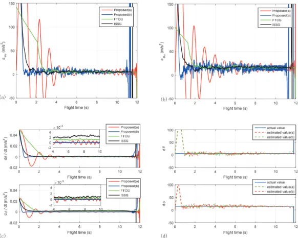
The design of the advanced guidance law against high maneuvering targets is always an active topic in the research field. In this paper, a finite-time convergent robust guidance law for interceptor missiles is proposed. Compared with the finite-time convergence guidance (FTCG) law [22] and input-to-state stability-based guidance (ISSG) law [23], the proposed law has better convergence characteristics.

The remainder of this paper is structured as follows. In Section 1, the planar dynamic model of target-missile relative motion is derived. Section 2 introduces a SMOB to estimate the target acceleration. The proposed robust SM guidance law is presented in Section 3, and its boundedness and stability are analyzed using the finite-time bounded function method and Lyapunov second method, respectively. Section 4 presents the simulation results, which demonstrate the effectiveness of the proposed guidance law. Finally, Section 5 concludes this paper.

2. Governing Equations

In real interception, the target-missile relative motion occurs in a spherical environment. Considering the axial symmetry of missile body, a guidance model can be set up in a plane to simplify the study. First, a planar model of the guidance process is built in part A; then, the spherical model is built in part B. Suppose the research object throughout this paper satisfies the following conditions:

I. The mass is uniformly distributed. II. No rolling or rolling rate is small enough.

III. Dynamic features are similar in every direction

perpendicular to the axis.

VI. Actuators respond rapidly enough.

Then, the missile can be considered a point mass.

A. Planar dynamics model of the guidance process

The planar dynamics model of target-missile relative motion is shown in Fig. 1.

A series of equations is given as follows according to Fig. 1. There are only some mistakes in equations：

1.

Please check the period（.）or periods（..）on the top of every letter.

eq（1）~ eq（6）should be changed as

r V _Tcos





_T





V_Mcos





_M





, (1)









sin sin / , T T M M V V r



_















_ (2) / , M a VM M   (3) / , T a VT T   (4) 2 _, Tr Mr r r



a a (5) 2r aT aM , r r r



    (6) eq（10）should be changed as





1 1/ 1 ˆ ˆT ˆ psgn ˆ M , q a h q q q q r



a        





1 2/ 2 ˆT ˆ psgn ˆ , a h q q q q     ₍₁₀₎ eq（14）should be changed as



1





ˆ 2 1



sgn

 



2



, cos M T M a 

_{ }

_ a r



k



s cs k 



 





1 sgn s cs . r







 (14) eq（17）should be changed as

V x

 





1

V x

 





3

V x

2

 



0.

₍₁₇₎ eq（27）should be changed as , (1)

There are only some mistakes in equations：

1.

Please check the period（.）or periods（..）on the top of every letter.

r V _Tcos





_T





V_Mcos





_M





, (1)











_















a a (5) 2r aT aM , r r r







1 1/ 1 ˆ ˆ ˆ psgn ˆ , T M q a h q q q q r



a        







1





ˆ 2 1



sgn

 



2



_{ }

_ a r



k



s cs k 



 





1 sgn_r s cs .







V x

 





1

V x

 





3

V x

2

 



0.

1.

Please check the period（.）or periods（..）on the top of every letter.

r V _Tcos





_T





V_Mcos





_M





, (1)











_















a a (5) 2r aT aM , r r r









a        





1 2/ 2 ˆ ˆ psgn ˆ , T a h q q q q     ₍₁₀₎ eq（14）should be changed as



1





ˆ 2 1



sgn

 



2



, cos M T M a  

_{ }

_ a r



k



s cs k 



 





1 sgn s cs . r







V x

 





1

V x

 





3

V x

2

 



0.

1.

Please check the period（.）or periods（..）on the top of every letter.

r V _Tcos





_T 





V_Mcos





_M





, (1)











_















a a (5) 2r aT aM , r r r









a        







1





ˆ 2 1



sgn

 



2



_{ }

_ a r



k



s cs k 



 





1 sgn s cs . r







V x

 





1

V x

 





3

V x

2

 



0.

where VT and VM are the missile velocity and target velocity,

respectively; aT and aM are the missile acceleration and target

acceleration, respectively; λ denotes the LOS angle; r denotes

the distance between the missile and the target; rM and rT

denote the trajectory inclination angles of the missile and target, respectively.

Take the derivatives of eq.(1) and eq.(2), respectively, with respect to time to obtain

1.

Please check the period（.）or periods（..）on the top of every letter.

r V _Tcos





_T





V_Mcos





_M





, (1)











_















a a (5) 2r aT aM , r r r









a        







1





ˆ 2 1



sgn

 



2



_{ }

_ a r



k



s cs k 



 





1 sgn s cs . r







V x

 





1

V x

 





3

V x

2

 



0.

1.

Please check the period（.）or periods（..）on the top of every letter.

r V _Tcos





_T 





V_Mcos





_M





, (1)











_















a a (5) 2r aT aM , r r r









a        







1





ˆ 2 1



sgn

 



2



_{ }

_ a r



k



s cs k 



 





1 sgn s cs . r







V x

 





1

V x

 





3

V x

2

 



0.

where aTr=aT sin(λ-rT) and aMr=aM sin(λ-rM) are the

accelerations along the LOS of the target and missile, respectively; aTλ=aT cos(λ-rT) and aMλ=aM cos(λ-rM) are the

accelerations perpendicular to the LOS direction of the target and missile, respectively.

Remark 1: For aerodynamic-force-controlled missiles, the acceleration in the velocity direction is always uncontrollable. Thus, only eq. (6) can be used to design the guidance law. In eq. (6),

5

the distance between the missile and the target;

M

 and _T denote the trajectory inclination angles

of the missile and target, respectively.

Take the derivatives of eq.(1) and eq.(2), respectively, with respect to time to obtain 2 Tr Mr r r



a a , (5) ₂ T M r a a r r r



    , (6) where _sin

_

_

Tr T T

a a   and aMr aMsin



  M



are the accelerations along the

LOS of the target and missile, respectively; _cos

_

_

T T T

a a   and aM aMcos



  M



are the accelerations perpendicular to the LOS direction of the target and missile, respectively. Remark 1: For aerodynamic-force-controlled missiles, the acceleration in the velocity direction is always uncontrollable. Thus, only eq. (6) can be used to design the guidance law. In eq. (6),

1

2

T

 



 



are two single points, but they are not the unstable points [24]. It is easy to see that

0 r 

is another single point from eq. (6), but because of the volume of the missile and target, in real interception, this issue will not occur. Thus, the following assumption makes important sense.

Assumption 1: During the procession of terminal guidance, the distance _r between the missile and the target has a range, i.e.,

min max

r  r r .

B. Spherical dynamics model of the guidance process

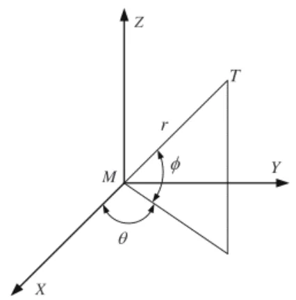
The spherical dynamics model of the target-missile relative motion is shown in Fig. 2.

are two single points, but they are not the unstable points [24]. It is easy to see that

r=0 is another single point from eq. (6), but because of the

volume of the missile and target, in real interception, this issue will not occur. Thus, the following assumption makes important sense.

Assumption 1: During the procession of terminal

guidance, the distance r between the missile and the target has a range, i.e., rmin<r<rmax.

B. Spherical dynamics model of the guidance process

The spherical dynamics model of the target-missile relative motion is shown in Fig. 2.

In Fig. 2, the original point is denoted as the gravity center of the missile, M and T are the missile and target, respectively;

r is the straight-line distance between the missile and the

4

the study. First, a planar model of the guidance process is built in part A; then, the spherical model is built in part B. Suppose the research object throughout this paper satisfies the following conditions:

I. The mass is uniformly distributed. II. No rolling or rolling rate is small enough.

III. Dynamic features are similar in every direction perpendicular to the axis. VI. Actuators respond rapidly enough.

Then, the missile can be considered a point mass.

A. Planar dynamics model of the guidance process

The planar dynamics model of target-missile relative motion is shown in Fig. 1.

Fig. 1 Planar model of target-missile relative motion A series of equations is given as follows according to Fig. 1.









cos cos T T M M r V   V   , (1)









sin sin / T T M M V V r _      _ , (2) / M aM VM   , (3) / T a VT T   , (4) where T

V and VM are the missile velocity and target velocity, respectively; aT and aM are

the missile acceleration and target acceleration, respectively;

_

denotes the LOS angle; _r denotes Fig. 1. Planar model of target-missile relative motion

Finite-Time Convergent Guidance Law Based on Second-Order Sliding Mode Control Theory

697

Paper