Deep learning-based household electric energy consumption forecasting

(1)

The Journal of Engineering

The 3rd Asian Conference on Artificial Intelligence Technology (ACAIT

2019)

Deep learning-based household electric

energy consumption forecasting

eISSN 2051-3305 Received on 14th October 2019 Accepted on 12th November 2019 E-First on 27th July 2020 doi: 10.1049/joe.2019.1219 www.ietdl.org

Jonghwan Hyeon

1

_{, HyeYoung Lee}

1

_{, Bowon Ko}

1

_{, Ho-Jin Choi}

1

1_{School of Computing, Korea Advanced Institute of Science and Technology, Daejeon, Republic of Korea}

E-mail: [email protected]

Abstract: With the advent of various electronic products, the household electric energy consumption is continuously increasing,

and therefore it becomes very important to predict the household electric energy consumption accurately. Energy prediction models also have been developed for decades with advanced machine learning technologies. Meanwhile, the deep learning models are still actively under study, and many newer models show the state-of-the-art performance. Therefore, it would be meaningful to conduct the same experiment with these new models. Here, the authors predict the household electric energy consumption using deep learning models, known to be suitable for dealing with time-series data. Specifically, vanilla long short-term memory (LSTM), sequence to sequence, and sequence to sequence with attention mechanism are used to predict the electric energy consumption in the household. As a result, the vanilla LSTM shows the best performance on the root-mean-square error metric. However, from a graphical point of view, it seems that the sequence-to-sequence model predicts the energy consumption patterns best and the vanilla LSTM does not follow the pattern well. Also, to achieve the best performance of each deep learning model, vanilla LSTM, sequence to sequence, and sequence to sequence with attention mechanism should observe past 72, 72, and 24 h, respectively.

1 Introduction

With the advent of various electronic products, the household electric energy consumption is continuously increasing, and therefore it becomes very important to accurately predict the household electric energy consumption. By predicting energy consumption accurately, the energy producer can generate and distribute the appropriate amount of power in advance, and prevent blackout when the amount of power production is less than the amount of power consumption. Consumers can also establish a reasonable power consumption plan.

Energy prediction models have been developed for decades with advanced machine learning technologies [1]. For example, recent studies on predicting energy consumption try to apply deep learning techniques to improve their prediction accuracy [2, 3].

Meanwhile, the deep learning models are still actively under study, and many newer models show the state-of-the-art performance. Therefore, it would be meaningful to conduct the same experiment with the latest deep learning model showing the state-of-the-art performance.

In this paper, we compare the vanilla long short-term memory (LSTM) model 4, which showed good performance in the model used in the previous study [3], with the sequence-to-sequence model and sequence-to-sequence model [5–7] with attention mechanism together, which have shown great performance recently. After the comparison of each model performance, then we find the optimal number of past observation data needed to forecast energy consumption. This experiment can carry out various time resolutions, and we design the experiment with 1-h resolution, which is the most useful in practice. Finally, in experimental data, we look for energy feature which fits best with our modern model.

This work is organised as follows: Section 2 introduces how deep learning approaches are used to forecast energy consumption. Our experiments are described in Section 3. Finally, we conclude this work by discussing some remaining issues in Section 4.

2 Methodology

In this section, we describe how deep learning approaches are used to forecast household electric energy consumption.

2.1 Overview

Household electric energy consumption is the total amount of energy consumed per unit time. So, to forecast energy consumption, we need to exploit models that can handle time-series data. In deep learning, the time-time-series data are normally dealt with recurrent neural networks (RNNs) because these networks can take a sequence of values and detect temporal relationships between the given values. Therefore, we focus on how to forecast energy consumption using various RNN architectures.

In this paper, we formalise the household electric energy consumption forecasting problem as follows:

• Given p past observations X = {xt−p+ 1, …, xt− 1, xt}. • Forecast p future values Y = x^

t+ 1, x^t+ 2, …, x^t+p , where t indicates an arbitrary time.

2.2 Vanilla LSTM

When an input sequence goes long, the conventional RNNs had a problem of losing the information at the beginning of the given sequence. To solve this problem, Hochreiter and Schmidhuber proposed an LSTM in 1997 [4]. Since LSTM controls the information flow through an input gate, an output gate and a forget gate, LSTM can prevent the problem of losing the information even the sequence becomes longer. At time step t, a state of the LSTM ht can be defined as follows:

ft= σg(Wfxt+ Ufht− 1+ bf) it= σg(Wixt+ Uiht− 1+ bi) ot= σgWoxt+ Uoht− 1+ bo

ct= ft∘ ct− 1+ it∘ σcWcxt+ Ucht− 1+ bc

ht= ot∘ σhct

where xt is the input vector to the LSTM at time step t, ft is the forget gate's activation vector, it is the input gate's activation vector, ot is the output gate's activation vector, ct is the cell state vector, the

J. Eng., 2020, Vol. 2020 Iss. 13, pp. 639-642

This is an open access article published by the IET under the Creative Commons Attribution-NoDerivs License (http://creativecommons.org/licenses/by-nd/3.0/)

(2)

initial values are c0= 0 and h0= 0 and the operator ∘ denotes the element-wise product.

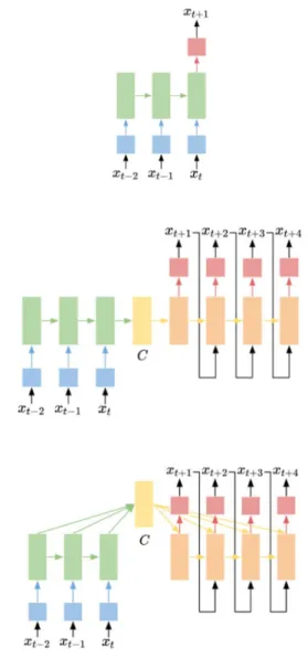
We design an LSTM network to forecast the household electric energy consumption by adopting many-to-one architecture that takes a sequence and produces a value. Since we are required to forecast a sequence of future values, we utilise the recursive multi-step forecasting strategy as follows (Fig. 1):

LSTM xk−p+ 1, …, xk− 1, xk = x^k+ 1 LSTM xk−p+ 2, …, xk, x^k+ 1 = x^k+ 2

⋮

LSTM xk, …, xk+p− 2, x^k+p− 1 = x^k+p

2.3 Sequence to sequence

Sequence-to-sequence architecture [5] consists of two RNNs. The first network called an encoder takes an input sequence and encodes the sequence into a context vector. That is the encoder summarises trends of the input sequence into the context vector. Then, the second network called a decoder takes the context vector and decodes the context vector into a corresponding sequence.

To forecast the household electric energy consumption, we design a sequence-to-sequence architecture as follows. As the sequence-to-sequence architecture naturally produces a sequence, we do not need to utilise any multi-step forecasting strategies:

Encoder xk−p+ 1, …, xk− 1, xk = C Decoder C = x^

k+ 1, x^k+ 2, …x^k+p

where C∈ ℝh_{is a context vector and h is the number of hidden} units (Fig. 2).

2.4 Sequence to sequence with attention mechanism

In the sequence-to-sequence architecture, the encoder should summarise all the information accurately into the one context vector. Thus, the context vector becomes the information bottleneck. To solve this problem, the sequence to sequence with attention mechanism has been proposed [8, 9].

In this architecture, the decoder does not rely on only one global context vector. Rather, a context vector is newly calculated using both the input sequence and the global context for each time step during the decoding process. Doing so, the decoder can focus only on certain parts of the input sequence, not on the entire input sequence (Fig. 3).

3 Experiments

3.1 Dataset

We used ‘Individual household electric power consumption dataset’ [10] from the UCI Machine Learning Repository. This dataset contains 2,075,259 measurements gathered in a house located in Sceaux (7 km of Paris, France) between December 2006 and November 2010 (47 months). The dataset contains global active power, sub-metering 1 which corresponds to the kitchen, metering 2 which corresponds to the laundry room, and sub-metering 3 which corresponds to an electric water heater and an air conditioner.

Fig. 1 Vanilla LSTM architecture

Fig. 2 Sequence-to-sequence architecture

Fig. 3 Sequence-to-sequence architecture with attention mechanism

640 J. Eng., 2020, Vol. 2020 Iss. 13, pp. 639-642

(3)

Since 1.25% of this dataset is missing, we filled these missing values with an average of measured values at the same time, in different years.

As this research aims at forecasting energy consumption, we calculated the active energy using the following formula. Then, these active energy values were averaged over an hour:

Active energy = Global active power × 1000_{60 − all sub − meterings}

Among 4 years, the values of the first 3 years were used as the train and validation dataset, and last year's values were used as the test dataset. In the train and validation dataset, 80% was used as the training dataset and 20% was used as the validation dataset.

3.2 Evaluation metric

To evaluate forecasting models, we measured the root-mean-square error (RMSE) on the test dataset:

RMSE = 1n_{i = 1}

∑

n Yi− Y^i2

To check overall performance of a forecasting model, as shown in Fig. 4, we moved a window one by one and measured an RMSE within the window. Then, we calculated an average of these RMSE values.

3.3 Implementation details

All architectures described in Section 2 were implemented using PyTorch [11]. All sequence-to-sequence models used LSTM as their RNN architecture, and teacher forcing was used when training them [12]. All models were initially trained by Adam optimiser [13], and then were trained further using the stochastic gradient descent with momentum [14]. In the sequence-to-sequence architecture with attention mechanism, attention scores were calculated according to the method proposed by Luong et al. [9] All hyper-parameters were selected through grid search on the validation dataset.

3.4 Comparison between architectures

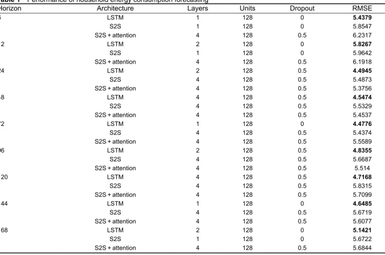
Table 1 shows the performance of household electric energy consumption forecasting. Horizon indicates how many observations are given. Among the three architectures, the vanilla LSTM shows the highest performance in all horizon cases.

Fig. 4 RMSE was measured within the sliding window

Table 1 Performance of household energy consumption forecasting

Horizon Architecture Layers Units Dropout RMSE

6 LSTM 1 128 0 5.4379 S2S 1 128 0 5.8547 S2S + attention 4 128 0.5 6.2317 12 LSTM 2 128 0 5.8267 S2S 1 128 0 5.9642 S2S + attention 4 128 0.5 6.1918 24 LSTM 2 128 0.5 4.4945 S2S 4 128 0.5 5.4873 S2S + attention 4 128 0.5 5.3756 48 LSTM 4 128 0.5 4.5474 S2S 4 128 0.5 5.5329 S2S + attention 4 128 0.5 5.4537 72 LSTM 1 128 0 4.4776 S2S 4 128 0.5 5.4374 S2S + attention 4 128 0.5 5.5589 96 LSTM 2 128 0.5 4.8355 S2S 4 128 0.5 5.6687 S2S + attention 4 128 0.5 5.514 120 LSTM 4 128 0.5 4.7168 S2S 4 128 0.5 5.8315 S2S + attention 4 128 0.5 5.7099 144 LSTM 1 128 0 4.6485 S2S 4 128 0.5 5.6719 S2S + attention 4 128 0.5 5.6077 168 LSTM 2 128 0 5.1421 S2S 1 128 0 5.6722 S2S + attention 4 128 0.5 5.6844 S2S: sequence to sequence.

Bold values represent the lowest RMSE value among architectures with the same horizon.

J. Eng., 2020, Vol. 2020 Iss. 13, pp. 639-642

(4)

Sequence-to-sequence architectures achieve similar performances regardless of the attention mechanism.

3.5 Comparison between horizons

When forecasting the energy consumption, it is important to choose the optimal time horizon for the model because the horizon largely affects the performance. In vanilla LSTM, the 72-h horizon achieves the best performance, while the 12-h horizon is lowest. In sequence-to-sequence architecture, higher horizons show higher performance than lower horizons.

3.6 Discussion

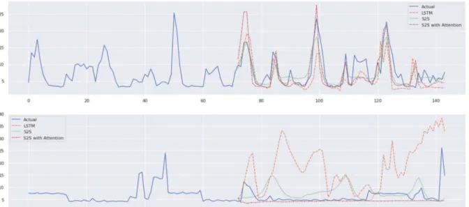
As shown in Table 1, the vanilla LSTM shows the best performance among all horizons according to RMSE values. However, as shown in Fig. 5, the vanilla LSTM often predicts completely different values when an unusual trend appears. In contrast, the sequence-to-sequence architectures predict the pattern-compliant values in the same situation.

4 Conclusion

This paper presented three methods to predict the energy consumption in a residential building. We compare energy prediction performance among three deep learning models which are vanilla LSTM, sequence to sequence, and sequence to sequence with attention mechanism. The vanilla LSTM showed the best performance when evaluated with the RMSE metric, but the sequence-to-sequence model seems to be pattern compliant. The optimal number of past observation data with the 1-h resolution is different among models. The vanilla LSTM is 72, sequence-to-sequence is 72, and sequence-to-sequence-to-sequence-to-sequence with attention is 24. We found that it is very difficult to forecast the energy consumption with no certain patterns such as metering 1 (kitchen), sub-metering 2 (laundry). None of the three models seems to predict these sub-meterings.

In future works, we will explore other evaluation metrics that can reflect situations as shown in Fig. 5. In addition, we will use

the date and time to conduct further research so that the model predicts trends that occur only at specific times.

5 Acknowledgments

This research was supported by the Korea Electric Power Corporation (grant number R18XA05).

6 References

[1] Suganthi, L., Samuel, A.A.: ‘Energy models for demand forecasting – a review’, Renew. Sust. Energy Rev., 2012, 16, (2), pp. 1223–1240

[2] Mocanu, E., Nguyen, P.H., Gibescu, M., et al.: ‘Deep learning for estimating building energy consumption’, Sustain. Energy Grids Netw., 2016, 6, pp. 91– 99

[3] Marino, D.L., Amarasinghe, K., Manic, M.: ‘Building energy load forecasting using deep neural networks’. IECON 2016 – 42nd Annual Conf. of the IEEE Industrial Electronics Society, Florence, Italy, 2016, pp. 7046–7051 [4] Hochreiter, S., Schmidhuber, J.: ‘Long short-term memory’, Neural Comput.,

1997, 9, (8), pp. 1735–1780

[5] Sutskever, I., Vinyals, O., Le, Q.V.: ‘Sequence to sequence learning with neural networks’. Advances in Neural Information Processing Systems, Montreal, Canada, 2014, pp. 3104–3112

[6] Mocanu, E., Nguyen, P.H., Gibescu, M., et al.: ‘Comparison of machine learning methods for estimating energy consumption in buildings’. Int. Conf. on Probabilistic Methods Applied to Power Systems (PMAPS), Durham, England, 2014, pp. 1–6

[7] Bontempi, G., Taieb, S.B., Le Borgne, Y.A.: ‘Machine learning strategies for time series forecasting’. European Business Intelligence Summer School, 2012, pp. 62–77

[8] Bahdanau, D., Cho, K., Bengio, Y.: ‘Neural machine translation by jointly learning to align and translate’, preprint, arXiv:14090473, 2014

[9] Luong, M.T., Pham, H., Manning, C.D.: ‘Effective approaches to attention-based neural machine translation’, preprint, arXiv:150804025, 2015 [10] Hebrail, G., Berard, A.: ‘Individual household electric power consumption

data set’. UCI Machine Learning Repository, 2012

[11] Paszke, A., Gross, S., Chintala, S., et al.: ‘Automatic differentiation in pytorch’. NIPS-W, California, USA, 2017

[12] Williams, R.J., Zipser, D.: ‘A learning algorithm for continually running fully recurrent neural networks’, Neural Comput., 1989, 1, (2), pp. 270–280 [13] Kingma, D.P., Ba, J.: ‘Adam: A method for stochastic optimization’, preprint,

arXiv:14126980, 2014

[14] Sutskever, I., Martens, J., Dahl, G., et al.: ‘On the importance of initialization and momentum in deep learning’. Int. Conf. on Machine Learning, Atlanta, USA, 2013, pp. 1139–1147

Fig. 5 Predicted household electric energy consumption (randomly sampled)

642 J. Eng., 2020, Vol. 2020 Iss. 13, pp. 639-642