Research Article
Design and Implementation of Spatial Operators and
Energy-Efficient Query Processing Strategy in Wireless Sensor
Network Database System
Chong sok Lim,
1Jeong-Hoon Lee,
2Minjee Park,
3and Soon J. Hyun
1,3 1Department of Information and Communication Engineering, KAIST, 373-1 Guseong-dong, Yuseong-gu,Daejeon 305-701, Republic of Korea
2Department of Creative IT Engineering, POSTECH, 77 Cheongam-Ro, Nam-gu, Pohang, Gyeongbuk 790-784, Republic of Korea 3Department of Computer Science, KAIST, 373-1 Guseong-dong, Yuseong-gu, Daejeon 305-701, Republic of Korea
Correspondence should be addressed to Soon J. Hyun; [email protected] Received 4 April 2014; Revised 15 August 2014; Accepted 17 August 2014 Academic Editor: Lei Shu
Copyright © 2015 Chong sok Lim et al. This is an open access article distributed under the Creative Commons Attribution License, which permits unrestricted use, distribution, and reproduction in any medium, provided the original work is properly cited. Database applications in wireless sensor networks very often demand data collection from sensor nodes of specific target regions. Design and development of spatial query expressions and energy-efficient query processing strategy are important issues for sensor network database systems. The existing sensor network database systems lack the needed sophistication for the space calculation of the target sensor nodes; hence, unnecessary query/data transmissions are required between the sensor nodes and the server. This paper describes our spatial operations and energy-efficient query processing methods that are designed and implemented in our sensor network database system called SNQL+𝑠. With a set of spatial operators based on geometric parameters, such as Envelope, NearBy, Distance, Direction, and set theoretic operators, SNQL+𝑠allows sensor network applications to easily specify the target space of interest. Our energy-efficient query processing strategy implements an in-network query management based on the lowest common ancestor (LCA) algorithm, so that the query processing cost for calculating the target spaces is greatly reduced by avoiding the need of heavy query/data transmissions between the base-station and target nodes. Performance evaluation shows that our proposed design and implementation of spatial query expressions and processing strategy achieve improved energy efficiency for database operations in the wireless sensor network.
1. Introduction
Sensor networks are increasingly used in a wide range of modern applications, including disaster management, preci-sion agriculture, healthcare, traffic management, and ecolog-ical monitoring as one of the most useful emerging
infor-mation management systems [1–5]. In many earlier
devel-opments of sensor networks, sensor nodes were viewed as network components; therefore, they were designed mainly to propagate stream data over a network to the base-station using preinstalled data aggregation instructions from the
network perspectives [6, 7]. From the data management
perspectives, on the other hand, a sensor network is viewed as a real-world resource of time-variant data in a sense similar to a huge database reservoir. By grafting the traditional database management perspectives to the sensor network, sensor
networks have become more functional in data processing so as to be able to serve a wider range of modern sensor network applications.
The typical procedure of query processing in a sensor network database system can be summarized as follows: (1) an application issues a query over to the sensor network; (2) the designated sensor nodes execute the query; and (3) data are aggregated along the topological alignment of networked sensor nodes back to the base-station, where the application processes them on the fly or stores them in a back-end database. A few works on sensor network database systems
have been reported [8–12].
The sensor nodes in a wireless sensor network have battery limitation and consume more energy for query/data transmission over the networked nodes than for data read-ing at the nodes. Therefore, how to reduce (and balance)
the energy consumption for query/data transmission is an important research issue. Query processing in wireless sensor networks exploits in-network processing methods and rout-ing plans in an effort to minimize and balance the battery consumption during the course of query/data transportation
[9,10,13].
Applications of database management in the sensor net-works typically require data collection from the nodes of some geographical areas of interest as a target space, such as an area damaged by forest fire, an area designated as the peak, an area of a given coordinate, and areas of an abrupt increase in traffic, north of a certain point. Reducing the energy consumption in the wireless sensor network is an important issue to achieve efficient data reading operations at individual sensor nodes and maintain energy balance for the entire sensor network as well. The design and development of spatial query operations and associated query processing strategies are important issues in sensor network databases for achieving energy-efficient data management.
Spatial queries in sensor network databases often have multiple targeting structures, such as “read temperatures from the regions where the humidity is lower than 10% in the west slope of the mountain.” This query indicates the first target space as “the west slope of the mountain” and the next target space is formed according to the humidity readings from the sensor nodes in the first target area. It seems that this query is intended to monitor and predict a possible forest fire.
A few sensor network database systems have been
designed [8–12]. However, for their limited spatial
expres-sions, they require multiple query disseminations and data collections by issuing a query to select sensor nodes of the first target region (i.e., the west slope in the above example) and another query to collect data from sensor nodes of the second target region(s) with humidity lower than 10% in the example. In our proposed approach, on the other hand, a single query with spatial operations manages multiple targeting by using an in-network query processing method so that the identification of subsequent target region(s) is done at some intermediate nodes called lowest common ancestor (LCA) nodes without traversing to and from the base-station. This paper presents our design and implementation of spatial operations and associated query processing algorithm in an effort to better support sophisticated demands of sensor network applications. We have designed spatial operators based on geometric parameters, such as Envelope, Nearby, Distance, and Direction, as well as binary spatial operators, such as Intersection, Union, and Difference in an attempt
to extend our previous sensor network database SNQL [8,
14]. We also have developed our query processing method
called LCA-based in-network query processing (in short, LCA-algorithm). We have defined a LCA node as one of the parent sensor nodes that minimally covers all the leaf nodes of the target region that participate in the query processing. At the LCA node, the new target region will be identified according to the data read from the nodes of the initial target region, and then the registered query at the LCA node is reformed and redisseminated for final reading without traversing to and from the base-station. Our proposed spatial
query expressions and LCA algorithm together will efficiently reduce the query processing cost in the wireless sensor network.
The contribution of this paper is summarized as follows. (i) We have extended our previous work on sensor
net-work query language SNQL [8,14] by incorporating
various spatial operators, so that more sophisticated expressions of target space are made possible in our
new system called SNQL+𝑠.
(ii) We designed an efficient query processing strategy by employing the concept of lowest common ancestor (LCA), which implements an efficient in-network query processing for spatial query operations.
The rest of this paper is organized as follows.Section 2
introduces related works, andSection 3describes the spatial
operators. Section 4 explains the LCA-based in-network
query processing algorithm.Section 5explains the
architec-ture of the SNQL+𝑠, and Section 6 shows the performance
evaluation. Finally, conclusions are given inSection 7.
2. Related Work
Madden et al. have proposed TinyDB which is a distributed query processing system running on the Berkeley mote
platform on top of TinyOS operating system [9]. It supports
acquisitional query processing (ACQP) that has the features
of when, where, and in what order the sensor nodes are sampled and which nodes should be included in processing a particular query. It also manages a semantic routing tree (SRT) to store a single one-dimensional interval, representing the range values beneath each of its children in each node. For example, when a query that has a spatial condition, such as “𝑥-coordinate > 100”, arrives at a node, the node checks
whether any child’s 𝑥-coordinate range value overlaps the
spatial condition of the given query. If so, it forwards the query down to the child nodes. Thus, SRT supports the effi-cient dissemination of queries and collection of query results over spatial conditions. However, since spatial expression is limited to disseminating a query only to target nodes with the coordinates in the query, multiple queries are needed if the intermediate query results are used as the conditions for the following queries as given in the aforementioned example. Di Felice et al. have extended TinyDB to support the spatial expression of queries by means of the longitude and
latitude of the nodes indicating their physical locations [15].
To apply spatial operation, the attributes of TinyDB are extended with longitude and latitude to create the precondi-tions for the georeferencing of the sensor nodes. The extended TinyDB enables the processing of some spatial operators, such as Distance, Inbox, and Beyondboundary. Among these operators, Inbox determines whether a node exists within a given envelope for identifying nodes in a physical space. For example, if one wants to read temperature from a
rect-angle(0, 0, 500, 500), “SELECT temperature FROM sensors
WHERE Inbox[0, 0, 500, 500]” is issued. However, since only
a few spatial operators are supported, there are limitations in expressing queries related to location information in a sensor
network. For instance, it does not support operators to find nodes in a designated direction and to find the node closest to a given position.
Kim et al. proposed Spatial TinyDB, which supports spa-tial data types and spaspa-tial operators by extending TinyDB by incorporating standard geospatial expressions proposed by
the Open Geospatial Consortium (OCG) [16,17]. The spatial
TinyDB supports spatial data types, spatial relation operators, spatial analysis operators, and spatial trajectory operators. Their spatial data types are managed in seven types: Point, LineString, Polygon, PolyhedralSurface, MultiPoint, Multi-LineString, and MultiPolygon. Also, eight spatial relation operators are given, such as Equals, Disjoint, Touches, Within, Overlaps, Crosses, Intersection, and Contains. Each relation operator receives two spatial objects and returns True or False as the output. Spatial analysis operators include six operators, such as Distance, Intersection, Difference, Union, Buffer, and Convexhull. Each receives two spatial objects and returns a new spatial object as the output. However, since the spatial data types are limited to expressing a region with the coordinates of area, it is not suitable to select an unfixed target region (e.g., the region where the humidity is lower than 10%), and thus it requires multiple queries if intermediate query results are used as the conditions for the following queries.
Yao et al. proposed the Cougar system, in which sensor data is periodically collected from the physical environment
and is represented by time series [10, 11]. They proposed
query processing over sensor data which are considered as a virtual relational database, so that a user can issue queries without knowing the physical characteristics of the sensor network. In Cougar, it is assumed that each sensor type has a standard abstract data type (ADT) representation which is used at all nodes. Sensors can be treated as ADT objects in query processing, and the user application manages a SQL-like interface through ADT. Here, the simplified schema of the sensor network database contains one relation R(loc point, floor int, s sensorNode), where loc is a point ADT that stores the coordinates of the sensor, floor is the floor where the sensor is located in the data warehouse, and sensorNode is a sensor ADT that supports the methods detectAlarmTemp(threshold). Here, the threshold is the threshold temperature above which abnormal temperatures are returned. For example, if one wants to generate a notification when two sensors within 5 yards of each other simultaneously measure an abnormal temperature, “SELECT R1.s.detectAlarmTemp(100), R2.s.detectAlarmTemp(100)
FROM R R1, R R2 WHERE $SQRT ($SQR(R1.loc.x −
R2.loc.x) + $SQR(R1.loc.y− R2.loc.y)) < 5” is issued.
How-ever, the location is stored in the front-end server for que-rying so that query processing takes place on the centralized database. Therefore, if intermediate query results are used as the conditions for the following queries, it also needs to disseminate multiple queries.
Shen et al. proposed SINA [12] which supports
SQL-like query and script using a language called Sensor Query
and Tasking Language (SQTL). This system is based on a
spreadsheet database where each attribute is referred to as a cell, and it incorporates a hierarchical clustering mechanism.
SQTL provides primitives for sensor hardware access (e.g., getTemperature, turnOn), location aware (e.g., isNeighbor, getPosition), and communication (e.g., tell, execute) prim-itives, as well as event handling. These scripts migrate from node to node depending on their parameters by the
sensor execution environment (SEE) located in each sensor
node. Then, the SEE examines all SQTL messages and performs the appropriate operation. For example, messages with “ALL NODES” are rebroadcasted to every sensor node, and those with “NEIGHBORS” are forwarded only to nodes that are one-hop-away neighbours in the sensor network. As in these examples, location is used for primitive operations, such as forwarding messages. Therefore, spatial operation does not work efficiently when multiple targets are used.
Amongst the studies related to spatial query processing in sensor networks, some attempt to utilize spatial indexing for query processing. Soheili et al. suggested Spatial Index
(SPIX), which applied R-Tree to sensor network [18]. In
that, a sensor node forms Minimum Boundary Area (MBA) that includes the location information of itself and of its descendant sensor nodes along the routing pass and manages these in the form of R-tree. The MBA is used to determine whether the spatial query, once received from a higher-level node for sensor data collection within a given area, should be passed to the lower-level nodes. Li et al. proposed back forwarding method, which uses SPIX mechanism for disseminating query and rearranging mechanism for return
route of the query result to base-station [19]. By restructuring
return path dynamically for the query result, they reduced the energy cost of aggregating the query result. Park et al. sug-gested Sectioned Tree, which divides the entire network into several squares that form local sections and in which the head node of a section manages the MBR to determine whether
to pass the spatial query [20]. Dyo and Mascolo investigated
a solution to reduce the energy consumption for creation
and management of spatial index [21]. They decomposed
the entire network into a set of disjoint hierarchical square cells, where each cell consists of four smaller cells. Then, they placed the cluster heads at fixed coordinates to reduce the algorithms and communications required to search for cluster heads. Our index management scheme is also
MBR-based algorithm for query processing as given inSection 5.2.
The minimum boundary rectangle (MBR) of subtrees for each sensor node is used for determining to pass the query down to the child nodes when the target space overlaps MBR of subtrees. No matter how index is managed, they lack the needed capability of managing multiple targeting in a single query if intermediate query results are used as the condition for finding the target space in the subsequent queries as given in the aforementioned example.
Sensor Network Query Language (SNQL) and its query
processor use SQL-like language structure and various query
processing functions running over Android [8, 14]. It is
designed to support instant queries, continuous queries, and event-based queries. SNQL implements various querying operations to reduce the energy consumption of sensor nodes by minimizing the amount of transactions in query/data propagations among sensor nodes while maintaining the computing capability. For example, conditional branching
(xi, yj) (xj, yj)
(xi, yi) (xj, yi)
Figure 1: SNQL+𝑠 envelope identified by the vertices (𝑥𝑖, 𝑥𝑗, 𝑦𝑖, 𝑦𝑗).
query provides a case-based branching mechanism in that the collection of sensor data is dynamically set based on the data values of the designated sensor nodes. The node-selection query supports a percentage-based node-selecting mechanism by WITHIN-clause for choosing only a certain number of participating nodes rather than using all nodes. Location-aware event detection query provides specification of the event monitoring region and the target region of sensor nodes from which the notified types of sensor data are collected through in-network query processing. Despite its sophisticated language expressions and query processing methods, the SNQL still lacks the needed capability of spatial query operations, and thus it suffers from the same inefficiency for spatial querying as other sensor network databases.
3. Spatial Operators for SNQL
+𝑠3.1. Design of SNQL+𝑠Space. In this section, the spatial
opera-tors of SNQL+𝑠 are introduced, by extending the previous
SNQL [8, 14] to support various space operations. A
geo-metric target space in SNQL+𝑠 is represented by a rectangle
called a SNQL+𝑠 envelope as the basic unit for spatial query
operation. The concept of the SNQL+𝑠 envelope is similar to
the ENVELOPE used in GIS [16]. Different from the GIS
ENVELOPE that returns the minimum bounding box for
a geometric object, our SNQL+𝑠 envelope identifies a group
of sensor nodes that together satisfy given condition(s) and returns a target space of interest.
The SNQL+𝑠 envelope is represented in the form:
{𝑠𝑝𝑎𝑐𝑒-𝐼𝐷, (𝑥𝑖, 𝑥𝑗, 𝑦𝑖, 𝑦𝑗)}, where space-ID is the
geome-tric space identifier, and (𝑥𝑖, 𝑥𝑗, 𝑦𝑖, 𝑦𝑗) is the space
nota-tion to denote the vertices of the envelope {(𝑥𝑖, 𝑦𝑖),
(𝑥𝑗, 𝑦𝑖), (𝑥𝑖, 𝑦𝑗), (𝑥𝑗, 𝑦𝑗)} as depicted inFigure 1.
The point of a location is also regarded as a type of a SNQL+𝑠 envelope with𝑖 = 𝑗. This implies that a single sensor
node may form an envelope as depicted in Figure 2 (step
1). Thus, all the SNQL+𝑠 spaces are expressed as SNQL+𝑠
envelopes so as to achieve closure property for the spatial query
operations.
Based on the feature of SNQL+𝑠 envelope to identify the
target regions, we have designed a few useful space operators as given in the following subsections.
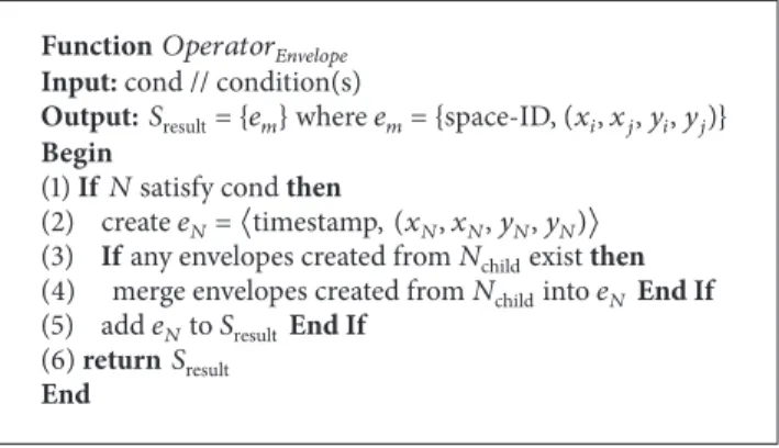
Function𝑂𝑝𝑒𝑟𝑎𝑡𝑜𝑟𝐸𝑛V𝑒𝑙𝑜𝑝𝑒 Input:cond // condition(s)
Output:𝑆result={𝑒𝑚} where 𝑒𝑚={space-ID, (𝑥𝑖, 𝑥𝑗, 𝑦𝑖, 𝑦𝑗)} Begin
(1) If𝑁 satisfy cond then
(2) create𝑒𝑁=⟨timestamp, (𝑥𝑁, 𝑥𝑁, 𝑦𝑁, 𝑦𝑁)⟩ (3) If any envelopes created from𝑁childexist then (4) merge envelopes created from𝑁childinto𝑒𝑁End If
(5) add𝑒𝑁to𝑆result End If
(6) return𝑆result
End
Algorithm 1: Procedure of Envelope operation.
3.2. Space Identification Operators
3.2.1. Envelope (Condition(s)). The Envelope operation will
result in a group (or groups) of sensors forming geometric space(s) together satisfying given condition(s). For example, a query: “find the space of sensor nodes where the temperature
is above 30 degrees” is expressed by Envelope (temp> 30).
SNQL+𝑠 envelopes are merged with adjacent ones.
Figure 2illustrates how leaf nodes (as the smallest envelopes)
are merged into a larger envelope. In step 1 ofFigure 2, eight
nodes (node-1 to node-8) satisfy the query condition so as
to form SNQL+𝑠 envelopes e1 to e8. Then, in step 2, the
SNQL+𝑠 envelopes e1, e2, and e3 are merged with e4, e5, and e6, respectively, and thus new enlarged SNQL+𝑠 envelopes e4, e5, and e6 are produced. This process repeats until that the
new enlarged SNQL+𝑠 envelope e7 is produced as shown in
step 3. On the other hand, e4 does not expand upwards as node-9 did not satisfy the given condition. Finally, e4, e7, and
e8 are sent to the base-station as the result of Envelope (temp
> 30) operation.
The procedure of Envelope operation is given in
Algorithm 1. 𝑁 denotes an arbitrary sensor node; the
child node of 𝑁 is defined as 𝑁child; the physical location
of 𝑁 is (𝑥𝑁, 𝑦𝑁). This operation receives the input
para-meter as cond (i.e., condition(s)) and returns a set of
geometric space 𝑆result = {𝑒𝑚}, where SNQL+𝑠 envelope
𝑒𝑚= {𝑠𝑝𝑎𝑐𝑒-𝐼𝐷, (𝑥𝑖, 𝑥𝑗, 𝑦𝑖, 𝑦𝑗)}. Here, space-ID is the
geome-tric space identifier, and (𝑥𝑖, 𝑥𝑗, 𝑦𝑖, 𝑦𝑗) denotes the vertices
of 𝑒𝑚 which identifies a group of sensor nodes that
toge-ther satisfy given condition(s). First, if node 𝑁 satisfies
the cond, a SNQL+𝑠 envelope 𝑒𝑁 is created in a form
⟨timestamp, (𝑥𝑁, 𝑥𝑁, 𝑦𝑁, 𝑦𝑁)⟩. Timestamp is used to
maintain the uniqueness of envelope, and(𝑥𝑁, 𝑥𝑁, 𝑦𝑁, 𝑦𝑁)
denotes the envelope notation of node𝑁 at (𝑥𝑁, 𝑦𝑁) with
𝑖 = 𝑗 (lines 1-2). If any envelopes created from 𝑁childexist,
those envelopes are merged into 𝑒𝑁 as a larger one (lines
3-4). Finally,𝑒𝑁is added to𝑆result(lines 5-6).
3.2.2. NearBy (𝑥𝑖, 𝑥𝑗, 𝑦𝑖, 𝑦𝑗). The NearBy operation
cre-ates and returns the geometric space of the nearest node to the specified target location in the form:
{𝑠𝑝𝑎𝑐𝑒-𝐼𝐷, (𝑥𝑖, 𝑥𝑗, 𝑦𝑖, 𝑦𝑗)}, where 𝑖 = 𝑗. The query is
Base-station 7 8 9 4 2 3 6 5 1 e1 e2 e3 e4 e5 e6 e7 e8 Step1 Node (temp> 30) (a) 7 8 9 4 2 3 6 5 1 e4 e5 e6 e7 e8 Step2 Base-station Node (temp> 30) (b) 7 8 9 4 2 3 6 5 1 e4 e8 e7 Step3 Base-station Node (temp> 30) (c) Figure 2: Formation of SNQL+𝑠 envelopes.
1 2 3 4 5 7 6 9 Step1 Base-station 8 Subtree of node-5 Subtree of node-6 10 x = 10, y = 20 (a) Step2 1 2 3 4 5 6 Base-station e1 e1 e1 e1 e1 e3 e2 x = 10, y = 20 (b) Figure 3: NearBy (10, 10, 20, 20).
the intermediate nodes along the query path will register
the query. Figure 3 shows how the query is propagated
to the node nearest to the target location. For example, a query: “find the space of the nearest sensor node from the coordinates (𝑥 = 10, 𝑦 = 20)” is expressed by NearBy (10, 10,
20, 20).
As shown in step 1 of Figure 3, nodes whose subtrees
include the given coordinates will receive and register the query of NearBy (10, 10, 20, 20). Thus, the query is passed along 1 to 6. On the other hand, 7 to node-10 do not receive the query since node-5 and node-6 did not send the query because their subtrees do not include the given
coordinates. In step 2, node-4 forms SNQL+𝑠 envelope e3 and
receives SNQL+𝑠 envelopes e1 and e2 formed by node-5 and
node-6, respectively. Then, node-4 passes e1 as the nearest one to the given target location to the base-station.
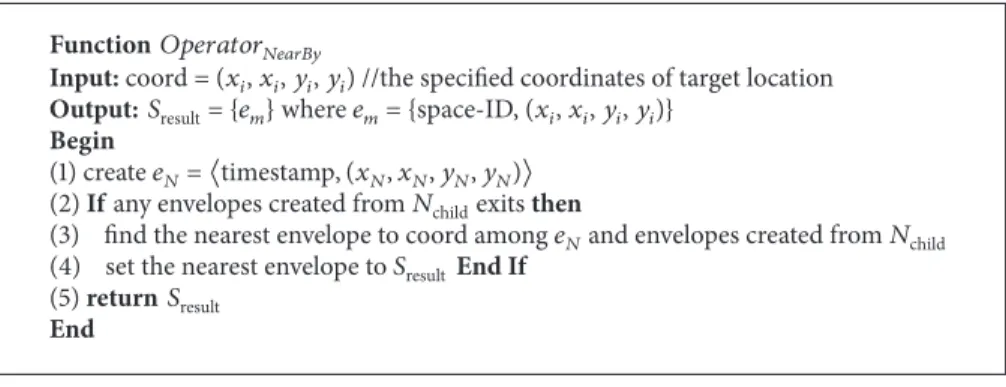
The procedure of NearBy operation is given in
Algorithm 2. This operation receives coord (i.e., coordinates
of a target location) as an input and returns a set of geometric
space𝑆result = {𝑒𝑚}, where 𝑒𝑚 = {𝑠𝑝𝑎𝑐𝑒-𝐼𝐷, (𝑥𝑖, 𝑥𝑖, 𝑦𝑖, 𝑦𝑖)}.
First, a SNQL+𝑠 envelope 𝑒𝑁 is created in a form
⟨timestamp, (𝑥𝑁, 𝑥𝑁, 𝑦𝑁, 𝑦𝑁)⟩ (line 1). If any envelopes
created from 𝑁child exist, they are compared with 𝑒𝑁 to
find the nearest one to coord. Then, the nearest envelope is returned (lines 2–5).
3.2.3. Distance (Envelope(s), Range Value). The Distance
operation identifies a geometric space for range value from
a designated geometric space. As mentioned inSection 3.1,
it is to be noted that a point of location is also expressed as
a SNQL+𝑠 envelope. For example, a query: “find the space
of sensor nodes which is 10 meter away from the geometric space where the temperature is above 30 degrees” is expressed
by Distance (Envelope (temp> 30), 10 m).
As shown in step 1 ofFigure 4, node-5 as a LCA node
Function𝑂𝑝𝑒𝑟𝑎𝑡𝑜𝑟𝑁𝑒𝑎𝑟𝐵𝑦
Input:coord = (𝑥𝑖,𝑥𝑖,𝑦𝑖,𝑦𝑖) //the specified coordinates of target location
Output:𝑆result={𝑒𝑚} where 𝑒𝑚={space-ID, (𝑥𝑖,𝑥𝑖,𝑦𝑖,𝑦𝑖)} Begin
(1) create𝑒𝑁=⟨timestamp, (𝑥𝑁, 𝑥𝑁, 𝑦𝑁, 𝑦𝑁)⟩ (2) If any envelopes created from𝑁childexits then
(3) find the nearest envelope to coord among𝑒𝑁and envelopes created from𝑁child (4) set the nearest envelope to𝑆resultEnd If
(5) return𝑆result End
Algorithm 2: Procedure of NearBy operation.
5 1 2 4 e1 e2 Step1 3 Base-station Node (temp> 30) (a) e2 Step2 Range Range 5 1 2 4
Node in expanded envelopes e1
3
Base-station
(b) Figure 4: Distance (Envelope (temp> 30), 10 m).
nodes satisfy the temperature condition. In step 2, node-5
produces expanded SNQL+𝑠 envelopes e1 and e2 according
to the given range value and sends the query to expanded SNQL+𝑠 envelopes e1 and e2.
The procedure of the Distance operation is given in
Algorithm 3. This function receives a set of geometric spaces
𝑆in = {𝑒1, 𝑒2, . . . , 𝑒𝑘}, where 𝑒𝑘 = {𝑠𝑝𝑎𝑐𝑒-𝐼𝐷, (𝑥𝑖, 𝑥𝑗, 𝑦𝑖, 𝑦𝑗)},
and a range value as input. It returns a set of geometric
spaces𝑆result= {𝑒1, 𝑒2, . . . , 𝑒𝑘}, where 𝑒𝑘is newly expanded
envelope of𝑒𝑘. To find the new envelope by the range value,
each envelope of𝑒𝑘is expanded by the(+/−) range value given
as the second input parameter (lines 1–3). Finally,𝑆result is
returned (lines 4-5).
3.2.4. Direction (Envelope(s), Direction Value). The Direction
operation identifies and returns a geometric space outside designated space in the given directions: NORTH, SOUTH, EAST, WEST, and their mixed orientations as well. For example, a query: “find the space of sensor nodes that are located in the WEST of some space where the temperature is above 30 degrees” is expressed by Direction (Envelope (temp > 30), WEST).
Figure 5 illustrates the operation. In step 1, node-5 as
a LCA node identifies SNQL+𝑠 envelopes e1 and e2 whose
member nodes have temperature values over 30 degrees. In step 2, node-5 finds e2 as the westernmost envelope of all
envelopes and thus returns the SNQL+𝑠 envelope e3 as the
result.
The procedure of Direction operation is given
in Algorithm 4. It receives a set of geometric spaces
𝑆in = {𝑒1, 𝑒2, . . . , 𝑒𝑘}, where 𝑒𝑘 = {𝑠𝑝𝑎𝑐𝑒-𝐼𝐷, (𝑥𝑖, 𝑥𝑗, 𝑦𝑖, 𝑦𝑗)},
and a direction value as input. It returns a set of geometric
space𝑆result = {𝑒𝑚}, where 𝑒𝑚 = {𝑠𝑝𝑎𝑐𝑒-𝐼𝐷, (𝑥𝑖, 𝑥𝑗, 𝑦𝑖, 𝑦𝑗)}.
After finding the closest envelope to the end of a given
direction from 𝑆in, the resulting geometric envelope 𝑒𝑁 is
identified in a given direction 𝐷. For example, when the
direction is given NORTH, the northernmost envelope in
𝑆in will be found and set to 𝜀. Then, envelope 𝑒𝑁 with a
space coordinates(𝑋min, 𝑋max, 𝜀 ⋅ 𝑦𝑗, 𝑌max) will be produced
as the resulting space whose𝑦𝑖is greater than𝜀 ⋅ 𝑦𝑗. Here,
𝑋max (𝑋min) denotes the maximum (minimum) value of
the x-coordinate of the region, and 𝑌max (𝑌min) denotes
the maximum (minimum) value of the y-coordinate of the region (lines 1–14).
3.3. Set Operators. Set operators are designed to identify the
sensor nodes of target spaces by using two operand spaces.
Function𝑂𝑝𝑒𝑟𝑎𝑡𝑜𝑟𝐷𝑖𝑠𝑡𝑎𝑛𝑐𝑒
Input:(1)𝑆in={𝑒1,𝑒2, . . . , 𝑒𝑘} where 𝑒𝑘={space-ID, (𝑥𝑖,𝑥𝑗,𝑦𝑖,𝑦𝑗)}
(2) ra // a range value
Output:𝑆result={𝑒1,𝑒2, . . . , 𝑒𝑘} where 𝑒𝑘is expanded envelope of𝑒𝑘 Begin
(1) For each𝑒𝑘in𝑆in
(2) Set envelope of𝑒𝑘with (𝑥𝑖− ra, 𝑥𝑗+ ra, 𝑦𝑖− ra, 𝑦𝑗+ ra) (3) EndFor
(4)𝑆result:= 𝑆in
(5) return𝑆result End
Algorithm 3: Procedure of Distance operation.
Function𝑂𝑝𝑒𝑟𝑎𝑡𝑜𝑟𝐷𝑖𝑟𝑒𝑐𝑡𝑖𝑜𝑛
Input:(1)𝑆in={𝑒1,𝑒2, . . . , 𝑒𝑘} where 𝑒𝑘={space-ID, (𝑥𝑖,𝑥𝑗,𝑦𝑖,𝑦𝑗)} (2)𝐷 // a direction value
Output:𝑆result={𝑒𝑚} where 𝑒𝑚={space-ID, (𝑥𝑖,𝑥𝑗,𝑦𝑖,𝑦𝑗)}
Begin
(1) Switch(𝐷) // find geometric space of direction operation (2) Case (𝐷 = 90) or (𝐷 = EAST):
(3) 𝜀 := easternmost 𝑒𝑘from𝑆in
(4) create𝑒𝑁=⟨timestamp, (𝜀 ⋅ 𝑥𝑗, 𝑋max, 𝑌min, 𝑌max)⟩ (5) Case (𝐷 = 270) or (𝐷 = WEST):
(6) 𝜀 := westernmost 𝑒𝑘from𝑆in
(7) create𝑒𝑁=⟨timestamp, (𝑋min, 𝜀 ⋅ 𝑥𝑖, 𝑌min, 𝑌max)⟩ (8) Case (𝐷 = 0) or (𝐷 = 360) or (𝐷 = NORTH) (9) 𝜀 := northernmost 𝑒𝑘from𝑆in
(10) create𝑒𝑁=⟨timestamp, (𝑋min, 𝑋max, 𝜀 ⋅ 𝑦𝑗, 𝑌max)⟩ (11) Case (𝐷 = 180) or (𝐷 = SOUTH):
(12) 𝜀 := southernmost 𝑒𝑘from𝑆in
(13) create𝑒𝑁=⟨timestamp, (𝑋min, 𝑋max, 𝑌min, 𝜀 ⋅ 𝑦𝑖)⟩ (14) End Switch
(15)𝑆result:= 𝑒𝑁 (16) return𝑆result
End
Algorithm 4: Procedure of Direction operation.
express more sophisticated target region. An example query is “get node IDs from the areas that are designated as multiple
spaces where the temperature is above 30∘C and/or/but not
where the humidity is lower than 10% in the west slope of the mountain.” For that query, Intersection, Union, and Difference operations are used to identify sensor nodes of new spaces. It is noted that Union and Difference operations produce multiple constituent subspaces for the best accuracy of the
result as shown in Figure 6. The given spaces are split to
subspaces as follows. In step 1, two operand spaces, such as
𝑆𝑎 = {𝑒𝑎1, 𝑒𝑎2} and 𝑆𝑏 = {𝑒𝑏1, 𝑒𝑏2}, are given. In step 2, after
cross product between each element of𝑆𝑎and that of𝑆𝑏,
inter-sect envelopes𝑒𝑖1and𝑒𝑖2are identified. In step 3, each element
envelopes of𝑆𝑎and𝑆𝑏are compared whether the spaces exist
surrounding𝑒𝑖1and𝑒𝑖2in the 8 direction: NORTH, SOUTH,
EAST, WEST, and their mixed orientations. Then existing
spaces form as𝑆𝑎 = {𝑒𝑠11, 𝑒𝑠12, 𝑒𝑠13, 𝑒𝑠23, 𝑒𝑠24, 𝑒𝑠25} and 𝑆𝑏 =
{𝑒𝑠15, 𝑒𝑠16, 𝑒𝑠17, 𝑒𝑠21, 𝑒𝑠27, 𝑒𝑠28}.
3.3.1. Intersection ((s1, s2)|Envelope(s), Envelope(s)). The Intersection operation takes two operand spaces either
explic-itly specified by space-IDs or implicexplic-itly specified by two
return values (i.e., SNQL+𝑠 envelopes) of spatial operations.
For the demonstration purpose we use an example query: “get node IDs from the intersection areas between where
the temperature is above 30∘C and where the humidity is
below 10% in the west slope of the mountain.” This query implies the possible executions for the multiple pairs of overlapping subspaces that satisfy the given conditions and
thus a set of subspaces (i.e., SNQL+𝑠 envelopes) will be
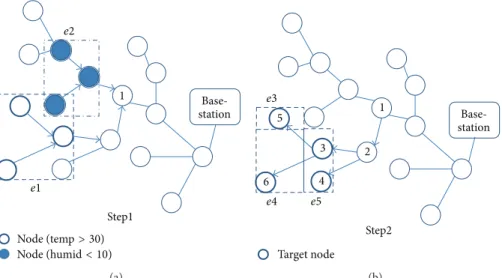
returned. Figure 7 illustrates an execution of Intersection
operation. In step 1, node-1 as a LCA node receives SNQL+𝑠
envelope e1 where the temperature is over 30∘C and SNQL+𝑠
envelope e2 where the humidity is below 10%. In step 2,
node-1 computes the intersect region of enode-1 and e2. Then, it creates
an SNQL+𝑠 envelope e3 and sends the query to the nodes of
4 5 1 3 2 e1 e2 Step1 Base-station Node (temp> 30) (a) Step2 5
Nodes in the west from the base envelope (e2)
e2 e3
Base-station
(b) Figure 5: Direction (Envelope (temp> 30), WEST).
Step1 ea1 eb1 eb2 ea2 (a) Step2 ea1 eb1 eb2 ea2 ei2 ei1 (b) Step3 ei2 ei1 es12 es11 es18 es13 es17 es14 es15 es16 es22 es21 es23 es27 es28 es24 es25 es26 (c) Figure 6: Procedure of producing multiple constituent subspaces.
3.3.2. Union ((s1, s2)|Envelope(s), Envelope(s)). The Union
operation takes two operand spaces either explicitly specified by space-IDs or implicitly specified by two return values (i.e., SNQL+𝑠envelopes) of spatial operations. An example query:
“get node IDs from the union areas where the temperature
is above 30∘C or where the humidity is below 10% in the
west slope of the mountain” is used. This example implies the possible execution of the multiple pairs of overlapping subspaces that satisfy the given conditions and, as the result,
a set of constituent subspaces (i.e., SNQL+𝑠 envelopes) will
be returned.Figure 8illustrates an example execution of the
Union operation. In step 1, node-1 as a LCA node receives
SNQL+𝑠 envelope e1 where the temperature is over 30∘C and SNQL+𝑠 envelope e2 where the humidity is below 10%. In step
2, node-1 computes the union area of e1 and e2 by splitting it based on the intersect area. Then, it creates e3 to e9 and sends the query to the sensor nodes of e3 to e9. It is to be noted that,
unlike the Intersection operation, the Union operation yields a set of constituent envelopes that together form the union of
two spaces as shown inFigure 8(step 2).
3.3.3. Difference ((s1, s2)|Envelope(s), Envelope(s)). The Dif-ference operation takes two operand spaces either explicitly
specified by space-IDs or implicitly specified by two return
values (i.e., SNQL+𝑠 envelopes) of spatial operations. An
example query: “get node IDs from the areas where the
temperature is above 30∘C but where the humidity is not
below 10% in the west slope of the mountain” is used. This example implies the possible execution of multiple pairs of overlapping spaces that satisfy the given conditions and,
as the result, a set of constituent subspaces (i.e., SNQL+𝑠
envelopes) will be returned. Figure 9illustrates an example execution of the Difference operation. In step 1, node-1 as a
1 Step1 e1 e2 Base-station Node (temp> 30) Node (humid< 10) (a) Step2 1 4 e3 Base-station Target node (b) Figure 7: Intersection (Envelope (temp> 30), Envelope (humid < 10)).
1 Step1 e1 e2 Base-station Node (temp> 30) Node (humid< 10) (a) Step2 2 1 3 4 5 8 7 6 9 e5 e7 e3 e4 e8 e9 e6 station Base-Target node (b) Figure 8: Union (Envelope (temp> 30), Envelope (humid < 10)).
is over 30∘C and SNQL+𝑠 envelope e2 where the humidity is
below 10%. In step 2, node-1 computes the area of difference between e1 and e2 by splitting it based on the common area.
Then, it creates SNQL+𝑠 envelopes e3, e4, and e5 and sends
the query to nodes in e3, e4, and e5. Similar to the Union operation, this operation yields a set of constituent envelopes that together form the resulting subspaces of the Difference
operation as shown inFigure 9(step 2).
The procedure of Set operation is given in Algorithm 5.
This function receives op name (i.e., operator name),𝑆𝑎 =
{𝑒1, 𝑒2, . . . , 𝑒𝑎} and 𝑆𝑏= {𝑒1, 𝑒2, . . . , 𝑒𝑏} as input, and it returns
a set of geometric spaces𝑆result = {𝑒1, 𝑒2, . . . , 𝑒𝑛}, where 𝑒𝑛 =
{𝑠𝑝𝑎𝑐𝑒-𝐼𝐷, (𝑥𝑖, 𝑥𝑗, 𝑦𝑖, 𝑦𝑗)}. First, when each envelope 𝑒𝑎in𝑆𝑎
overlaps with envelope𝑒𝑏 in𝑆𝑏, an intersect envelope𝑒𝑖 is
created in a form⟨timestamp, (𝑥𝑖, 𝑥𝑗, 𝑦𝑖, 𝑦𝑗)⟩ (lines 1–4). By
comparing it in 8 directions (i.e., NORTH, SOUTH, EAST,
WEST, and their mixed orientations), 𝑒𝑎 is split into each
direction-positioned constituent envelope when if𝑒𝑎 exists
next to 𝑒𝑖 on each direction. Then, those envelopes form
𝜀𝑎 = {𝑒1, 𝑒2, . . . , 𝑒𝑘}. Also, 𝑒𝑏 is split in the same manner.
Here, the constituent envelopes are identified by the position
of𝑒𝑖. In the case ofFigure 8,𝑒3is created as an intersecting
envelope and then𝜀𝑎 = {𝑒7, 𝑒8, 𝑒9} and 𝜀𝑏 = {𝑒4, 𝑒5, 𝑒6} are
created surrounding𝑒3, whereas envelopes are not created
in the positions of north-west and south-east from𝑒3(lines
5-6). If op name is “Intersection,”𝑒𝑖 is added to𝑆result (line
7). If op name is “Difference,”𝜀𝑎 is added to𝑆result (line 8).
If op name is “Union,”𝜀𝑎,𝜀𝑏, and𝑒𝑖are added to𝑆result(line
9). If overlap does not exist,𝑒𝑎 is added to𝑆result when the
op name is “Difference.” Otherwise,𝑒𝑎 and𝑒𝑏 are added to
𝑆result when the op name is “Union” (lines 10–12). Finally,
1 Step1 e1 e2 Base-station Node (temp> 30) Node (humid< 10) (a) Step2 2 1 5 4 3 6 e3 e4 e5 Target node Base-station (b)
Figure 9: Difference (Envelope (temp> 30), Envelope (humid < 10)).
Function𝑂𝑝𝑒𝑟𝑎𝑡𝑜𝑟𝑆𝑒𝑡𝑂𝑝𝑒𝑟𝑎𝑡𝑜𝑟𝑠 Input:(1) op name
(2)𝑆𝑎={𝑒1,𝑒2, . . . , 𝑒𝑎} where 𝑒𝑎={space-ID, (𝑥𝑖,𝑥𝑗,𝑦𝑖,𝑦𝑗)} (3)𝑆𝑏={𝑒1,𝑒2, . . . , 𝑒𝑏} where 𝑒𝑏={space-ID, (𝑥𝑖,𝑥𝑗,𝑦𝑖,𝑦𝑗)}
Output:𝑆result={𝑒1,𝑒2, . . . , 𝑒𝑛} where 𝑒𝑛={space-ID, (𝑥𝑖,𝑥𝑗,𝑦𝑖,𝑦𝑗)} Begin
(1) For each𝑒𝑎in𝑆𝑎 (2) For each𝑒𝑏in𝑆𝑏
(3) Ifenvelope of𝑒𝑎overlap that of𝑒𝑏then
(4) create intersect envelope𝑒𝑖=⟨timestamp, (𝑥𝑖, 𝑥𝑗, 𝑦𝑖, 𝑦𝑗)⟩
(5) create𝜀𝑎={𝑒1,𝑒2, . . . , 𝑒𝑘} where 𝑒𝑘is constituent envelope of𝑒𝑎by splitting𝑒𝑎surrounding𝑒𝑖 (6) create𝜀𝑏={𝑒1,𝑒2, . . . , 𝑒𝑘} where 𝑒𝑘is constituent envelope of𝑒𝑏by splitting𝑒𝑏surrounding𝑒𝑖 (7) If(op name = “Intersection”) then add𝑒𝑖to𝑆resultEnd If
(8) If(op name = “Difference”) then add𝜀𝑎to𝑆resultEnd If
(9) If(op name = “Union”) then add𝜀𝑎,𝜀𝑏,𝑒𝑖to𝑆resultEnd If
(10) Else
(11) If(op name = “Difference”) then add𝑒𝑎to𝑆result End If
(12) If(op name = “Union”) then add𝑒𝑎,𝑒𝑏to𝑆resultEnd If
(13) End If (14) EndFor (15) EndFor
(16) remove redundant envelopes from𝑆result (17) return𝑆result
End
Algorithm 5: Procedure of SetOperators operation.
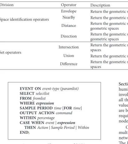
and𝑆𝑏, are removed from𝑆result(line 16).Table 1summarizes
the spatial operators in SNQL+𝑠.
3.4. Spatial Expressions in SNQL+𝑠. In this section, SNQL+𝑠 is introduced, which extends SNQL (Sensor Network Query
Language) [8,14] to be able to support the spatial operators.
The original SNQL was designed based on SELECT-FROM-WHERE structure and supports instant queries,
continu-ous queries, and event-based queries. Algorithm 6 shows
the basic structure of the original SNQL. SELECT-clause describes the attributes that correspond to the data to be collected from each sensor node. FROM-clause specifies the
initial target space for query dissemination. WHERE-clause describes the selection condition(s). EVENT ON specifies predefined events for the following query to be executed when the event takes place. SAMPLE PERIOD specifies various temporal notations for data collection. OUTPUT ACTION defines the sensor action to be performed when event or selection condition(s) are met. WITHIN-clause specifies the percentage of the nodes out of all the partic-ipating sensor nodes in the query processing, and CASE WHEN allows branching of query actions according to the situational conditions. More details are referred to in
Table 1: Spatial operators in SNQL+𝑠.
Division Operator Description
Space identification operators
Envelope Return the geometric spaces that satisfy a given condition
NearBy Return the geometric space that is the nearest to the specified point of location Distance Return the geometric spaces that satisfy within the given distance from the given
geometric spaces
Direction Return the geometric space that satisfies the given direction from the given geometric spaces
Set operators
Intersection Return the geometric spaces that lie in the intersection area of the given geometric spaces
Union Return the geometric spaces that lie in the union area of the given geometric spaces Difference Return the geometric spaces that lie in the difference area of the given geometric
spaces
EVENT ONevent-type (paramlist) SELECTselectlist
FROMfromlist
WHEREexpression
SAMPLE PERIODtime [FOR time]
OUTPUT ACTIONcommand
WITHINpercentage
CASE WHENevent| expression
THENAction| Sample Period | Within END;
Algorithm 6: The structure of SNQL.
To add spatial operators to the SNQL [8,14], the
expre-ssion in the WHERE-clause and WHEN-clause is extended as
described inAlgorithm 7. More specifically,<SpatialFunc> is
added to<SQLSimpleExp> of <Expression> so that the
spa-tial operators previously explained can be used.
<Spati-alFunc> consists of <Envelope>, <NearBy>, <Distance>, <Direction>, <Intersection>, <Union>, and <Difference>. <Envelope> is expressed as a combination of attributes (e.g., temperature), operators (e.g., “>”, “<”, or “=”), and constants. <NearBy> is expressed as integer values representing the
coordinates 𝑥 and 𝑦. <Distance> expresses the operator
selected from the elements of<SpatialFunc> and a constant
indicating the distance.<Direction> expresses the operator
selected from the elements of<SpatialFunc> and a constant
indicating the direction.<Intersection> consists of
combi-nations of <SpatialFunc> entities used to obtain the
inter-section.<Union> consists of combinations of <SpatialFunc>
entities used to obtain the union area.<Difference> consists
of combinations of<SpatialFunc> entities used to obtain the
difference area. <envelope>, <attribute>, <operator>, and
<constant> are fundamental attributes, whose descriptions are thus not necessary.
4. LCA: In-Network Query
Processing Algorithm
Sensor network queries often involve multiple phases of data reading in a single query task. The example query given in
Section 1“read the temperatures from the regions where the humidity is lower than 10% in the west slope of the mountain” involves two separate tasks: (1) read the humidity values from all the nodes in the west slope and (2) read the temperature values from the nodes in spaces where the humidity values are below 10%. In the existing systems, this operation would require two traversals between the base-station and the target nodes of the designated spaces.
Our proposed query processing algorithm enables the multiple phases of querying tasks to be handled by an in-network node called lowest common ancestor (LCA) node. The LCA node is one of the intermediate parent nodes which distributes the query to more than two child nodes for the first time and minimally covers all the child nodes of the target space. It has been designed to play the role of in-network query reformation and redissemination for the multiple reading tasks. This query processing algorithm will efficiently reduce the energy consumption of wireless sensor nodes incurred by unnecessary transmissions of multiple queries/data between the base-station (i.e., root node) and the target nodes.
The procedure of finding the LCA node is as follows. Each node along the query path manages two parameters
(#Ancestormax send, #Childsend). The former describes the
maximum number of child nodes to which its ancestor nodes send the query, and the latter describes the number of child nodes to which it passes the query further. The LCA node
is identified for a node when its #Childsendvalue becomes
greater than 1 for the first time along the query path.
Figure 10(a) illustrates how a LCA node is determined for the example query to the first target space. N01, as the base-station, receives the query and the Planner of Query Processor finds N02 as the receiver node toward the target space. Here, since N01 does not have a parent,
#Ancestormax sendbecomes 0. And, as it passes the query only
to N02, #Childsend becomes 1. In this manner, N03, N04,
N05, and N06 positioned in the query path to the first target
will have (#Ancestormax send = 1, #Childsend = 1). N07
receives the query from N06 and passes the query down to two child nodes so that the number of child nodes, for the
first time, becomes greater than 1 that is (#Ancestormax send=
⟨Expression⟩::=⟨SQLAndExp⟩ (“OR” ⟨SQLAndExp⟩)
⟨SQLAndExp⟩::= ⟨SQLRelationalExp⟩ (“AND” ⟨SQLRelationalExp⟩)
⟨SQLRelationalExp⟩::=⟨SQLSimpleExp⟩ | ⟨SQLExpressionList⟩ | ⟨SQLInClause⟩ | ⟨SQLBetweenClause⟩ ⟨SQLExpressionList⟩::=⟨SQLSimpleExp⟩ (“,” ⟨SQLSimpleExp⟩)
⟨SQLSimpleExp⟩::=⟨AggregateFunc⟩ | ⟨Count⟩ | ⟨NUMBER⟩ | ⟨STRING⟩ | ⟨BIND⟩ | ⟨SpatialFunc⟩ ⟨SpatialFunc⟩::=⟨Envelope⟩ | ⟨Nearby⟩ | ⟨Intersection⟩ | ⟨Union⟩ | ⟨Difference⟩ | ⟨Distance⟩ | ⟨Direction⟩ ⟨Enkelope⟩::=“ENVELOPE (“⟨attribute⟩ ⟨operator⟩ ⟨constant⟩”)”
⟨NearBy⟩::=“NEARBY (“⟨envelope⟩”)”
⟨Intersection⟩::=“INTERSECTION (”⟨SpatialFunc⟩ “,” ⟨SpatialFunc⟩ “)” ⟨Union⟩::=“UNION (”⟨SpatialFunc⟩ “,” ⟨SpatialFunc⟩ “)”
⟨Difference⟩::=“DIFFERENCE (”⟨SpatialFunc⟩ “,” ⟨SpatialFunc⟩ “)” ⟨Distance⟩::=“DISTNACE (”⟨SpatialFunc⟩ “,” ⟨constant⟩ “)” ⟨Direction⟩::=“DIRECTION (”⟨SpatialFunc⟩ “,” ⟨constant⟩ “)” ⟨enkelope⟩::=“(”⟨integer⟩ “,” ⟨integer⟩ “,” ⟨integer⟩ “,” ⟨integer⟩ “)” ⟨attribute⟩::=⟨string⟩
⟨operator⟩::=“>” | “<” | “=” | “<>” | “>=” | “<=” ⟨constant⟩::=⟨integer⟩ | ⟨float⟩ | ⟨string⟩
Algorithm 7: Spatial expression in SNQL+𝑠.
LCA N02 (1, 1) N03 (1, 1) N04 (1, 1) N05 (1, 1) N06 (1, 1) N07 (1, 2) Base-station N01(0, 1) (first target)
The west slope
(a) (second target) LCA Base-station Humidity< 10% (b) Figure 10: In-network query process with LCA node.
for the query, which is the lowest intermediate node that minimally covers all nodes of the target space (i.e., the west slope).
In Figure 10(b), the LCA node carries out a query task for data collection from the final target nodes (i.e., the nodes with humidity values lower than 10% within the initial target space). For this, the LCA node plays the key role of identifying the final target nodes and redisseminates the subsequent query task to the nodes (i.e., temperature reading).
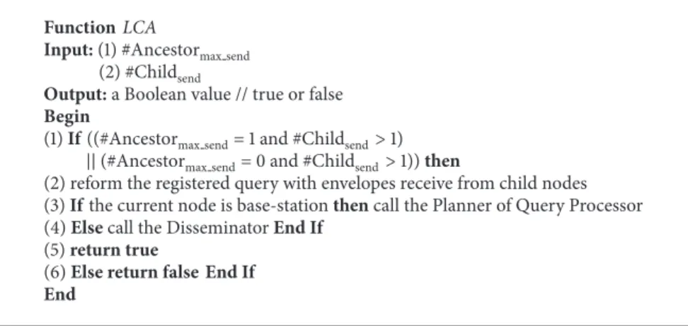
The procedure of LCA operation is given inAlgorithm 8.
This function receives #Ancestormax sendand #Childsendas the
input and returns True or False according to decision whether current node is LCA node or not. First, the registered query is reformed with envelopes received from its child nodes, if the current node satisfies following conditions: (1) for nodes
(#Ancestormax send = 1, #Childsend > 1) and (2) for
base-station (#Ancestormax send = 0, #Childsend > 1) (lines
1-2). Then, the Planner of Query Processor (or Disseminator) is called to disseminate the reformed query. And, true is returned (lines 3–5). If current node is not LCA node, false is returned (line 6).
5. Architecture
5.1. Overview. This section describes the architecture of our
sensor network database system. It consists of functional
components of the base-station as the SNQL+𝑠 server and
sensor nodes as illustrated in Figure 11. Upon receiving a
query, the Query Processor parses the query, plans execution, and sends the parsed query out to the network manager. It uses the metadata about the nodes and their connectivity (i.e., topology) to determine the pathway to the target nodes. The nodes along the hierarchical pathway to the sensor nodes of the initial target region will register the parsed query as the ancestor nodes for the target nodes, and one of the nodes will play the LCA role for identifying the new target nodes when multiple space operations apply. The executors of the nodes in the target space execute the query and return the
data toward the SNQL+𝑠 server along the ancestor nodes.
The Event Manager at the sensor node manages the events query registered at the target nodes, and the Action Manager manages the actions (e.g., beeping, beckoning, etc.) that need to be executed when the query condition is satisfied.
FunctionLCA
Input:(1) #Ancestormax send
(2) #Childsend
Output:a Boolean value // true or false
Begin
(1) If ((#Ancestormax send= 1 and #Childsend> 1)
|| (#Ancestormax send= 0 and #Childsend> 1)) then
(2) reform the registered query with envelopes receive from child nodes (3) If the current node is base-station then call the Planner of Query Processor (4) Else call the Disseminator End If
(5) return true
(6) Else return false End If
End
Algorithm 8: Procedure of LCA operation.
Node Node Base-station Catalog Parser Planner Executor Network manager Sensor network Query/data Node Network manager Sensing module Action module Query/data Query processor Catalog Disseminator Executor Query processor Event manager Action manager
Figure 11: System architecture of sensor network database using SNQL+𝑠.
The Network Manager passes the parsed query down to the nodes of the target region, receives the query result, and returns them to its parent node. Finally, the base-station postprocesses the collected sensor data into a form requested by the given query before giving them out to the application.
5.2. Metadata Management. The metadata of SNQL+𝑠, such as attribute types, location information, and
mini-mum boundary rectangle (MBR) of sensor nodes are used
during the query processing. Each node manages the metadata of directly connected child nodes in the form:
{(𝑥𝑖, 𝑦𝑖), (𝑁𝑜𝑑𝑒𝐼𝐷, {𝑠𝑒𝑛𝑠𝑜𝑟𝑇𝑦𝑝𝑒})}, where (𝑥𝑖, 𝑦𝑖) denotes the
coordinates of its child nodes and(𝑁𝑜𝑑𝑒𝐼𝐷, {𝑠𝑒𝑛𝑠𝑜𝑟𝑇𝑦𝑝𝑒})
denotes their nodeIDs and sensor types. Also, the metadata of its subtrees are described in the form:
{(𝑥𝑖, 𝑥𝑗, 𝑦𝑖, 𝑦𝑗), {𝑠𝑒𝑛𝑠𝑜𝑟𝑇𝑦𝑝𝑒}}, where (𝑥𝑖, 𝑥𝑗, 𝑦𝑖, 𝑦𝑗) denotes
the vertices as its MBR and {𝑠𝑒𝑛𝑠𝑜𝑟𝑇𝑦𝑝𝑒} denotes sensor
types of nodes in the subtree.Figure 12shows an example of
metadata management. Circles indicate sensor nodes, and the dotted line represents the region of the subtree as a MBR.
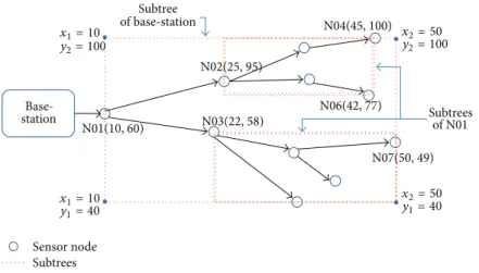
The base-station manages “⟨(10, 60), (𝑁01, {𝑠𝑒𝑛𝑠𝑜𝑟𝑇𝑦𝑝𝑒})⟩” as the metadata of the directly connected node and “⟨(10, 50, 40, 100), {𝑠𝑒𝑛𝑠𝑜𝑟𝑇𝑦𝑝𝑒}⟩” as the metadata of its sub-tree. Also, senor node N01 manages “⟨((25, 95), (𝑁02, {𝑠𝑒𝑛𝑠𝑜𝑟𝑇𝑦𝑝𝑒})), ((22, 58), (𝑁03, {𝑠𝑒𝑛𝑠𝑜𝑟𝑇𝑦𝑝𝑒}))⟩” as meta-data of the directly connected child nodes and “⟨((25, 45, 77, 100), {𝑠𝑒𝑛𝑠𝑜𝑟𝑇𝑦𝑝𝑒}), ((22, 50, 40, 58), {𝑠𝑒𝑛𝑠𝑜𝑟𝑇𝑦𝑝𝑒})⟩” as the metadata of its subtrees. In this manner, N02 manages the metadata of the directly connected two child nodes and two subtrees including MBR. Here, the MBR of subtree is used for determining to pass the query down to the child nodes when the target space overlaps MBR of subtrees. This metadata is created at the time of construction of the sensor network. When a node is added or deleted, the metadata is reconstructed by updating its parent and child nodes.
6. Performance Evaluation
6.1. Test Data and Environment. In this section, the
Base-station Sensor node N01(10, 60) N02(25, 95) N03(22, 58) N04(45, 100) N06(42, 77) Subtrees N07(50, 49) Subtree of base-station Subtrees of N01 x1= 10 y2= 100 x1= 10 y1= 40 x2= 50 y2= 100 x2= 50 y1= 40
Figure 12: An example of managing metadata.
Table 2: Simulation parameters.
Type Parameter Value
Network and nodes
Number of nodes 10,000
Sampling count of each node 1,000
Network range 1,000 m∗ 1,000 m
Time to sensing (s) 1
Network topology Tree
Transmit energy (mA) 10.40
Receive energy (mA) 9.30
Energy consumption [9] Processor, active (mA) 5.00
Processor, idle (mA) 0.001
Sensing energy (mA) 0.5
evaluated based on the energy efficiency. We used the Intel
Berkeley Research lab data [22] to generate random sensing
data as follows: normal distributions with a mean of 22.07 and a standard deviation of 3.662 for temperature data; a mean of 39.29 and a standard deviation of 7.162 for humidity data; and a mean of 390.87 and a standard deviation of 534.39 for illumination data. The number of nodes is set to 10000, and the sampling count of each node is set to 1000. Energy consumption of sensor network is caused by transmission,
reception, processing, and sensing of queries and data [9].
Table 2summarizes the simulation parameters.
All the experiments were conducted with a simulator which was programmed internally in Java and was extended
version of our previous work [8,14,23].
6.2. Experiments and Results. The efficiency of LCA-based
spatial operations is evaluated by two experiments for two typical spatial operations of multiple targeting: operation for identifying intermediate target region and operation for targeting multiple regions, respectively.
Experiment 1. A test query for identifying a new target region
according to the data result from the initial target space. In this experiment, we measured the amount of energy consumption for two different query processing methods:
Base-station R1 R2 R3 R4 R5
Figure 13: Area of target nodes varying the position of region.
one with LCA-based spatial operation and the other without the operation. This is measured by varying the distance of
target region from the base-station as shown inFigure 13.
The query used for this experiment is as follows.
“Get NodeID and light value of nodes from the intersecting area between an area with tempera-ture above T∘C and another area with the humid-ity below H% within the area of(𝑥1, 𝑥2, 𝑦1, 𝑦2).”
0 5 10 15 20 25 30 35 40 45 R1 R2 R3 R4 R5 Ener g y co n sum p tio n (mA)
Cumulative energy consumption
Without spatial operation With LCA-based spatial operation
×105
Figure 14: Varying the position of target region.
SELECTNodeID, light
FROMsensors
WHERE𝑠1(𝑥1, 𝑥2, 𝑦1, 𝑦2)
ANDIntersection (Envelope (temp> T∘C), Envelope
(humid< H%))
Multiple queries are needed when spatial operations with
LCA algorithm are not supported as in SNQL [8, 14] as
follows:
A SELECT NodeID, 𝑥, 𝑦 FROM sensors WHERE 𝑥 ≥
𝑥1 AND𝑥 ≤ 𝑥2 AND𝑦 ≥ 𝑦1 AND𝑦 ≤ 𝑦2 AND
(temp> T∘C)
B SELECT NodeID, 𝑥, 𝑦 FROM sensors WHERE
𝑥 ≥ 𝑥1 AND𝑥 ≤ 𝑥2 AND𝑦 ≥ 𝑦1 AND𝑦 ≤ 𝑦2
AND (humid< H%)
C SELECT NodeID, light FROM sensors WHERE
𝑥 ≥ 𝑥11AND𝑥 ≤ 𝑥22AND𝑦 ≥ 𝑦11AND𝑦 ≤ 𝑦22
The base-station will calculate the intersecting areas from
the results of query A and query B and then obtains the
NodeID and light value from queryC.
The multiple query executions to identify intermediate target regions and the extra spatial operation (i.e., INTER-SECT) at the base-station will consume energy and give application designer an extra programming overhead. On the
other hand, SNQL+𝑠uses sophisticated spatial expressions in
a single query and executes the spatial operations using the LCA algorithm. This will greatly improve energy efficiency and programming convenience.
Figure 14 shows the result of the experiment. Obvi-ously, as the distance of target region from the base-station increased, the number of intermediate nodes to send the final query results to the base-station also increased. Moreover, the gap of energy consumption between two curves becomes larger as our spatial operators with LCA-based processing algorithm effectively reduce multiple query/data transmis-sions between the base-station and querying nodes.
Experiment 2. A test query for identifying multiple target
regions.
In this experiment, we observe the amount of energy consumption by varying the number of target regions (denoted
by the number of target regions: 𝑁region) and the ratio of
participating nodes in the resulting target region (denoted by
selectivity:𝑁select).
The query used for this experiment is as follows.
“Get NodeID and light value of nodes in the area of(𝑥𝑎1, 𝑥𝑎2, 𝑦𝑎1, 𝑦𝑎2) or the area of (𝑥𝑏1, 𝑥𝑏2,
𝑦𝑏1, 𝑦𝑏2).”
Multiple queries are needed when spatial operators with LCA-based query processing algorithm are not supported as
in SNQL [8,14] as follows:
A SELECT NodeID, light FROM sensors WHERE
𝑥 ≥ 𝑥𝑎1AND𝑥 ≤ 𝑥𝑎2AND𝑦 ≥ 𝑦𝑎1AND𝑦 ≤ 𝑦𝑎2
B SELECT NodeID, light FROM sensors WHERE
𝑥 ≥ 𝑥𝑏1AND𝑥 ≤ 𝑥𝑏2AND𝑦 ≥ 𝑦𝑏1AND𝑦 ≤ 𝑦𝑏2
The multiple query executions in sending the queries to multiple target regions will consume energy and give application designer an extra programming overhead.
The above query is expressed in SNQL+𝑠as follows:
SELECTNodeID, light
FROMsensors
WHERE Union (𝑠1(𝑥𝑎1, 𝑥𝑎2, 𝑦𝑎1, 𝑦𝑎2), 𝑠2(𝑥𝑏1, 𝑥𝑏2,
𝑦𝑏1, 𝑦𝑏2))
SNQL+𝑠 uses spatial expressions in a single query and
executes the spatial operations using the LCA algorithm. This will greatly improve energy efficiency and programming convenience.
It is to be noted that our proposed set-theoretic spatial operations returns multiple regions to minimize the ratio of irrelevant sensor nodes in the target region (refer back to
Section 3.3).
Figures 15(a), 15(b), and 15(c) show how the number
of target regions affects the performance of two different query processing methods. Given three different ratios of
participating nodes in target nodes as selectivity factor𝑁select,
we measured the energy consumption of query processing for the different numbers of target regions. From the results, we found that the number of target regions gives rise to multiple query operations when spatial operator functions are not provided in the former queries. The single query expression and LCA-based in-network query processing method in the latter avoid the multiple traffics between the base-station and querying nodes.
Summarizing the above performance evaluation, our
proposed spatial query operators in SNQL+𝑠are found
effi-cient by avoiding unnecessary multiple query operations and programming overhead to identify the nodes of target spaces. Our LCA-based in-network query processing method mini-mizes the unnecessary query/data traffics between the base-station and the target nodes. Also, the sophisticated design of various spatial operators results in improved efficiency with their enhanced accuracy of target regions.
2 3 4 5 6 Ener g y co n sum p tio n (mA)
Cumulative energy consumption
Without spatial operation With LCA-based spatial operation 0 5 10 15 20 25 30 35 ×105 Nregion (a)𝑁select= 0.01 2 3 4 5 6
Cumulative energy consumption
Ener g y co n sum p tio n (mA) 0 5 10 15 20 25 30 35
Without spatial operation With LCA-based spatial operation
Nregion
×105
(b)𝑁select= 0.05
Cumulative energy consumption
2 3 4 5 6 Ener g y co n sum p tio n (mA) 0 5 10 15 20 25 30 35
Without spatial operation With LCA-based spatial operation
Nregion
×105
(c)𝑁select= 0.09
Figure 15: Cumulative energy consumption varying𝑁regionand𝑁select.
7. Conclusion
Since the sensor nodes in wireless sensor networks are deployed typically in a wide range of geographical regions, the geometric characteristics of nodes (such as topology, distance between nodes, and upwards/downwards directivity) will have to be closely considered for various applications. Obvi-ously, application will require reading sensor data of some regions of interest as target spaces of queries. Well-designed spatial query operations will achieve energy efficiency for the sensor nodes and the entire network as well. Existing query languages of sensor network databases lack needed sophisti-cation of specifying target regions and energy-efficient query processing strategies.
In this paper, the operators applicable to sensor networks were referred among the widely used standard GIS oper-ators and interpreted to suit the sensor network environ-ment. Then, these were categorized into space identification
operators and set operators, followed by the suggestion of
SNQL+𝑠, a query language that utilizes these operators. Space
identification operators are those that group the sensor nodes
in the area of interest according to condition. Set operators are those that create new geometric spaces from the spatial
relationships between geometric spaces given by the query or found in the query. The sophisticated design of those spatial operators results in improved efficiency of precise return of target regions.
We have designed LCA-based query processing algorithm for various spatial operations. With the algorithm, unneces-sary query/data transmissions between the base-station and the sensor nodes of target regions are avoided by using the notion of LCA nodes. The performance evaluation of our
proposed scheme implemented in SNQL+𝑠 showed superior
energy efficiency over our previous system without spatial operations.
Conflict of Interests
The authors declare that there is no conflict of interests regarding the publication of this paper.
Acknowledgment
This research was supported by the R&D Program supervised by the Institute for Information & Communications Technol-ogy Promotion (IITP), Korea (IITP-2014-044-041-002).