Development of Population Estimation Model based on 2.5D+ Building Dataset

Development of Population Estimation Model based on

2.5D+ Building Dataset

Kim, Byeongsun

_{· Jeon, Haechan}

_{· Lee, Heeseok}

The purpose of this study is to develop a model for estimating population to the lowest spatial level based on 2.5D+ building dataset, which can be more easily acquired than high-quality raster dataset such as a lidar DSM. We applied the model to Anyang City, GyeongGi-Do, with 2020 total population of 551,296, and tested the validation of the developed model through a linear regression model. The validation results showed that there wasn't a statistically significant difference between the estimated and reference population data. In addition, we found that in the case study, the discrepancies between the reference and estimated data revealed a systematic overestimation according to the building types and concentration of high-rise buildings. Therefore, a systematic approach to improve the quality of the population estimation should be investigated with considering the spatial distribution of estimation error.

Keywords : Population Estimation, 2.5D+ Building Dataset, Spatial Distribution, Lidar DSM, Linear Regression Model

1. Introduction

The knowledge of how many people live in a certain geographic area or political-administrative unit is valuable information. So population distribution data on a fine scale are of great significance in many areas including public health, emergency evacuation, disaster management, resource allocation, urban planning, market research, and transportation route design.

Such data, normally derived from demographic surveys

(e.g. census data), were aggregated into political units represented by irregular polygons. Although this method obtains accurate population information, it presents the information of population distribution in an aggregated way, sometimes due to confidentiality like personal information, which may hinder more accurate population-based analyses. In addition, choropleth maps have some other limitations, including the inaccuracy caused by periodic changes of the boundary of enumeration units, time lag between data collection and publication, and the

Received 2021. 03. 16, Revised 2021. 03. 25, Accepted 2021. 04. 05

1) Corresponding Author, Assistant Professor, Dept. Smart City Engineering, Anyang University (E-mail: [email protected]) 2) Dept. Urban Information Engineering, Master’s Course Student, Anyang University (E-mail: [email protected]) 3) Dept. Urban Information Engineering, Master’s Course Student, Anyang University (E-mail: [email protected])

https://doi.org/10.7848/ksgpc.2021.39.2.65 Original article

This is an Open Access article distributed under the terms of the Creative Commons Attribution Non-Commercial License (http:// creativecommons.org/licenses/by-nc/3.0) which permits unrestricted non-commercial use, distribution, and reproduction in any medium,

modifiable areal unit problem (MAUP)4)_.

In order to address the shortcomings of aggregate census data, several researchers have developed interpolation approaches for estimating areal population counts to raster-based population density surfaces, which is a process of spatial disaggregation. That is, it transforms data from source zones (e.g. census units) of known values to target zones (e.g. grid units or land use zones) with unknown ones.

These interpolation methods can be divided into two groups: simple interpolation and intelligent interpolation(Okabe and Sadahiro, 1997). Simple interpolation methods include all data transferring approaches that do not use ancillary data. In contrast to simple methods, intelligent interpolation methods involve integration with ancillary information to shed light on the internal variation of population density within each aggregation unit(Kim, 2009). Various data sources have been used as ancillary information. Examples include nighttime satellite imagery using the visible near-infrared (IR) band(Dobson et al., 2000; Sutton et al., 2001), housing distribution data (Moon and Farmer, 2001), land property parcel data(Luo, 2005), and land cover data derived from classified satellite imagery(Langford and Unwin, 1994; Holt et al., 2004; Reibel and Agrawal, 2007). Among those, land cover dataset is the most commonly used, given that it is highly correlated with population density.

On the other hand, all these methods rely on 2D datasets containing areas of land use or land cover zones. The simplest approaches rely on the total area of residential zones derived from land use data in a region. These methods perform reasonably well in homogeneous areas, but they exhibit significant errors in areas where buildings have a great variation in the number of stories(Biljecki et al., 2016). In fact, several researchers have indicated that the volume of buildings and floorspace provide a strong cue for its population. For instance, Lu et al.(2011) use multiple regression models to perform a study in Denver, Colorado,

based on both footprint areas and building volumes. Lwin and Murayama(2009) and Alahmadi et al. (2013) estimate the number of floors from an elevation dataset, and multiply it with the footprint area to get the approximate internal area of the apartments. Their results indicate that the volume-based approach gives more accurate results than the area of the footprints due to heterogeneous building morphologies. It can be observed that these studies have commonly used high-quality raster dataset such as a lidar DSM (Digital Surface Model) to derive a building's volume. However, it is quite difficult to acquire the dataset needed to apply the volume-based methods to the other regions because it usually takes a lot of time and cost to create the high-quality DSM dataset. Therefore, despite the frequent indication that volume-based methods can improve on the estimates of area-based methods, the methods which existing studies have suggested are a limitation in estimating the population of large-scale areas.

This paper thus attempts to estimate population to the lowest spatial level based on 2.5D+ building dataset, which can be easily acquired, instead of the DSM dataset. In order to achieve the aim of this study, there are three research objectives identified: (1) review the methods for population estimation with GIS (Geographic Information System) data and techniques; (2) present the population estimation model based on 2.5D+ building dataset; (3) perform a case study of Anyang city, both for the experiments and the validation of the model.

2. Methods for Population Estimation

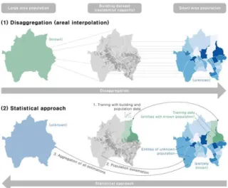
GIS and demography have long been closely related, and GIS techniques are ubiquitous in mapping, analyzing, and filling gaps in demographic data. Generally, the GIS techniques for estimation of population are divided into two groups, disaggregation(areal interpolation such as simple and intelligent interpolation) and statistical modeling approach(Fig. 1):

4) The modifiable areal unit problem (MAUP) is a source of statistical bias that is common in spatially aggregated data, or data grouped into regions or districts where only summary statistics are produced within each district, especially where the districts chosen are not suitable for the data (Jensen, J.R., Jensen, R.R, 2013).

Fig 1. Two groups of GIS techniques for population estimation (1) Statistical modeling approach analyzes the relationships between population and socio-economic variables associated with the population density, e.g. landuse, proximity to transportation network, and distance from the central business district. The deduced relationships are then applied to estimate the population count of unknown areas. In this approach multiple linear regression is most commonly used. The advantage of the bottom-up approach is that a sampling census has to carried out for only a small area. It is useful when only the population of a subset (e.g. a city) of a large area (e.g. a province) is known.

(2) Disaggregation method is a top-down approach where the population of a large administrative unit is distributed across smaller units, usually by weighting it according to different factors which hint at the population. This study uses three different indicators: building footprint area, floorspace, and building volume. This approach is typically used when the population of a large entity is known (e.g. a city), but the one of its composing entities is not known (e.g. its neighborhoods).

The disaggregation method, which is used in this paper,

is especially useful when the smaller units are political subdivision of the larger unit often found in choropleth maps, because such regions may contain variations in the population density

3. Materials

The study area is Anyang City, GyeongGi-Do, with 2020 total population of 551,296. It encompasses 2 census tracts (Manan-gu, Dongan-gu), and more detailed 31 dongs5)_.

The data of dong level administrative units joined with the 2020 Census data in ESRI shape format were acquired via SGIS(Statistical Geographic Information Service)6)_.

As mentioned before, this study uses 2.5D+ building dataset to overcome the limitations of building dataset derived from DSM in the case of estimating population. In general, 2.5D modeling is used in terrain modeling - the height is only an attribute that is used for example for visualization, while 2.5D+ modeling is an extension of the previous concept, but vertical faces are also allowed (Fig. 2). This is used in “block-shaped” models of building exteriors where roofs are horizontal planes with a height assigned; walls represented as vertical planes are reconstructed by extrusion(Ledoux and Meijers, 2010)

Fig . 2.5D terrain model(bottom) and 2.5D+ terrain model with a building(Top)

The 2.5D+ building dataset in estimating population is an ancillary dataset. This information is used to assist interpolation of data from the original source zones to new target zones (e.g. building unit). As ancillary dataset, the 2.5D+ building dataset of the study area was acquired for this purpose via National Spatial Data Infrastructure Portal7)_{. The building dataset was produced}

5) Gu (concept of district) is similar to boroughs in some Western countries and divided into dong (concept of neighborhoods). 6) SGIG Website : https://sgis.kostat.go.kr/

by joining the building layer in 1/5,000 digital map ver 2.0 with the Building Registers data in e-AIS (Internet Architectural Administration Information System). Thus, the information necessary for population estimation such as building's story, building's usage types (residential, commercial etc.) can be identified in the 2.5D+ building dataset (see Fig. 3).

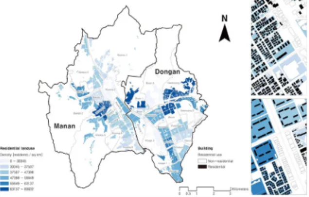
Fig. 3. Datasets used in this study: population density(residents/sq.km) of residential areas (Left) and 2.5D+ building dataset joined with the Building

Registers data in e-AIS (Right)

4. Methods and Validation of Population

Estimation

4.1 Population estimation methods

The general hypothesis used in this paper, and in related work, is simple: the larger the building, the more people reside in it. In addition, we have to consider only residential buildings, because the occupancy of a building depends on its type, e.g. a factory can be very large but at the same time it house zero inhabitants. Therefore, only residential buildings must be taken into account.

Based on the above discussions, the residential buildings in the study area were extracted from the dataset and the buildings volume was calculated by multiplying the area of each footprint by the corresponding building height. According to the number of stories in the dataset, a reference height was obtained by multiplying the number of stories with 3m, which is regarded as the average height of one story. This calculation was aggregated at the study area (SA) level,

as in Eq. (1):   



where RBVSA corresponds to the total residential building

volume of the study area, RBAi to the i-th residential building volume, RBHi to the i-th residential building height, and n denotes the total number of residential buildings found in the study area. In accordance with a method proposed by Almeida et al. (2011), the population estimates were realized based on the calculation of the habitable surface (HS).

Fig. 4. Example of HS calculation

As shown in Fig. 3, the HS of an i-th residential building is given by the ration of the i-th residential building volume (RBVi) to the average height from floor to ceiling (HFCi), as in Eq. (2):

     (2)

where HFC is set to 3m.

To estimate residential population at the Si level in 2020 (ERPSI2020), the aggregated value of HS per Dong (HSSI2020) was multiplied by a population density factor (PDSI2020), as in Eq. (3):

ERPSI2020=HSSI2020×PDSI2020 (3) In this study, PDSI2020 was calculated using net-residential area instead of the gross area including non-residential area to avoid greatly underestimating ERPSI2020.

4.2 Population estimation validation

In order to validate the estimated residential population, we compared our results to the population reference data through a simple linear regression given by:

    (4)

where  is the population reference data for the i-th

Dong;  is the estimated population from the result of this

work;  is the intercept;  is the angular coefficient; and

 is the random error term, with E ()=0 and Var ()=.

We expect that the reference population and the estimated population in this work are equivalent, and thus we assume that  is equal to zero and  is equal to 1. These hypotheses

are tested using Student’s t-test (Neter et al., 1996; Kim et al., 2010)

5. Results and Discussion

According to the research design, a case study was carried out for the study area which is the Anyang City, GyeongGi-Do, with 2020 total population of 551,296.

Tables 1 presents the Residential Buildings Volume (RBVdong2020), the Habitable Surface (HSdong2020), the Residential Population Density (RPDdong2020), the Estimated Residential Population (ERPdong2020), and the Reference Population Data (RPDdong2020) per Dong district, grouped according to the Gu districts to which they belong. The discrepancy between the estimated and reference data at the Dong level is shown in Table 1.

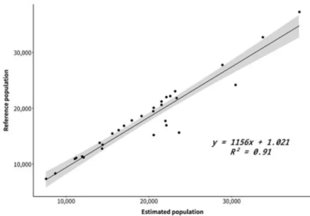
Fig. 5 shows the linear regression performed in regard to the estimated and reference population data (R² =0.91; t =316.5; p <0.001). The t-test indicated that there wasn't a statistically significant difference between reference and estimated population.

The estimated population presented on average 1,350 inhabitants more than the reference data. The discrepancies between the reference and estimated data reveal a systematic overestimation in our calculations, as shown in Table 1. The total estimated population (598,706 inhabitants) for the study

area is 8.6% more than the reference population (551,296 inhabitants).

In order to observe spatial distribution of the errors, we calculated NRMSE (Normalized Root Mean Squared Error)8) _{values and produced an error map as shown in Fig. 6.}

Fig. 5. Linear regression for estimated and reference population data

Fig. 6. The study area is divided into two types: new city(Dongan-gu) and old city(Manan-gu). Box A and B in Fig. 6 show the difference of the spatial distribution of estimation error between the new city(top-right) and the

old city(bottom-right)

In Fig. 6, box A is high-density residential buildings area in which many housing buildings like high-rise apartments are located. Beside box B, one of the medium-density residential buildings area, is an area where residential buildings have a great variation in low to high-rise height. Fig. 6 shows that

the errors of box B were relatively smaller than those of the box A on the area of high population density as well as high-rise apartments.

These errors can be explained by uncertainties introduced when calculating buildings volume by the 2.5D+ building dataset, which have particularly inaccurate values about

building’s height. In general, the height values, which were obtained by multiplying the number of stories with 3m, tend to be overestimated, as compared with the values of measured heights(Liang et al 2016). It means that the size of the model errors is more likely to be increased in the residential areas with the higher concentration of high-rise buildings, because Table 1. RBV, HS, RPD and Discrepancies between ERP and RPD

Gu Dong RBV(㎥) HS(㎡) RPD(inh/㎡) ERP RPD Discrepancies

Manan Anyang 1 257,983 773,949 0.05565 14,356 12,729 1,627 Anyang 2 494,079 1,482,236 0.04475 22,111 21,861 250 Anyang 3 559,474 1,678,423 0.03034 16,977 16,835 142 Anyang 4 143,456 430,369 0.05287 7,585 7,285 300 Anyang 5 412,451 1,237,352 0.02677 11,040 10,840 200 Anyang 6 404,264 1,212,793 0.05336 21,572 21,085 487 Anyang 7 233,183 699,548 0.07006 16,336 15,957 379 Anyang 8 300,556 901,667 0.03740 11,241 11,028 213 Anyang 9 533,352 1,600,055 0.03364 17,944 17,711 233 Seoksu 1 548,219 1,644,656 0.03751 20,562 19,929 633 Seoksu 2 645,109 1,935,327 0.05239 33,796 32,612 1,184 Seoksu 3 260,166 780,497 0.05400 14,049 13,736 313 Bakdal 1 373,225 1,119,676 0.04183 15,612 15,399 213 Bakdal 2 544,979 1,634,936 0.04254 23,184 22,940 244 sub-total 5,710,495 17,131,486 0.04304 246,364 239,947 6,417 Dongan Bisan 1 493,264 1,479,791 0.04740 23,379 21,724 1,655 Bisan 2 256,899 770,696 0.04707 12,091 11,127 964 Bisan 3 583,952 1,751,856 0.03278 19,144 18,528 616 Buheung 353,046 1,059,137 0.06232 22,001 17,664 4,337 Daran 240,674 722,023 0.05023 12,089 11,183 906 Gwanyang 1 729,532 2,188,597 0.05235 38,187 37,168 1,019 Gwanyang 2 348,607 1,045,821 0.05874 20,477 19,396 1,081 Burim 345,681 1,037,042 0.08363 28,910 27,547 1,363 Pyeongchon 279,911 839,732 0.07360 20,602 15,113 5,489 Pyeongan 482,882 1,448,647 0.06314 30,488 24,139 6,349 Gwiin 446,094 1,338,283 0.04959 22,124 16,870 5,254 Hogye 1 292,845 878,535 0.02970 8,699 8,238 461 Hogye 2 478,725 1,436,174 0.04495 21,517 20,524 993 Hogye 3 817,037 2,451,111 0.02767 22,605 22,064 541 Beomgye 314,666 943,997 0.07544 23,691 15,484 8,237 Sinchon 243,251 729,754 0.05923 14,409 13,334 1,075 Galsan 321,879 965,638 0.03706 11,929 11,246 683 sub-total 7,028,945 21,086,834 0.04920 352,343 311,349 41,024 Total 12,739,440 38,218,321 0.04631 598,706 551,296 47,440

the errors of building heights measured on 2.5D+ dataset can directly affect the estimation results of the model.

As future works for leading to more accurate population estimation, it would be worthwhile to investigate the influence of errors according to the quality and LoD (Levels of Detail) types of the input data when using volume-based approaches in population estimation.

6. Conclusion

This research developed a model to estimate residential population using 2.5D+ building dataset. The dataset was used in the model intended to incorporate information on buildings volume. Although the dataset obtained from 1/5,000 digital map haven’t satisfactory elevation accuracy in comparison with Lidar data (DSM, DTM), they are not only easily acquired but also utilized as the estimating population to the lowest spatial level(e.g. building level).

We applied the model to Anyang City, GyeongGi-Do, with 2020 total population of 551,296, and tested the validation of the developed model through a linear regression model. The validation results showed that there wasn't a statistically significant difference between the estimated and reference population data. However, we found that in this case study, the discrepancies between the reference and estimated data revealed a systematic overestimation. In particular, these errors appeared significant overestimation in the areas of high population density as well as high-rise apartments. These areas tend to be overestimated because of uncertainties introduced when calculating buildings volume by the 2.5D+ building dataset, which have generally inaccurate values about building’s height.

For future work, it would be worth noting that the spatial distribution of estimation error is one of the most important things affecting the accuracy of the model significantly. Therefore a systematic approach to improve the quality of the population estimation according to the building types of residential areas and the spatial distribution of estimation error should be investigated.

The derived data on the number of residents on a finer scale is beneficial for a multitude of applications such as disaster management, infrastructure planning, assessing exposure to

noise, optimizing network coverage (e.g. television) to cover more people, estimating energy consumption and in urban simulations. Furthermore, the algorithms we suggested in this paper would be also applied in the 3D City Model of the Digital Twin for Land, which is one of the national work projects in the Korean New Deal.

Acknowledgements

This work was supported by a grant (21DRMS-B147287-04) for the development of customized realistic 3D geospatial information update and utilization technology based on consumer demand, funded by MOLIT, Korea.

References

Alahmadi, M., Atkinson, P., and Martins, D. (2013), Estimating the spatial distribution of the population of riyadh, saudi arabia using remotely sensed built land cover and height data, Computers, Environment and Urban Systems, Vol. 41, pp. 167-176.

Almeida, C.M., Oliveira, C.G., Rennó, C.D., and Feitosa, R.Q. (2011), Population estimates in informal settlements using object-based image analysis and 3D modeling, ICEO-IEEE Earthzine, Accessed 24 February 2013. Biljecki, F., Ohori, K.A., Ledoux, H., Peters, R., and Stoter,

J. (2016), Population estimation using a 3D city model: a multi-scale country-wide study in the netherlands, PLoS ONE, Vol. 11, No. 6, pp. 1-22.

Dobson, J.E., Bright, E.A., Coleman, R., Durfee, R.G., and Worley, B.A. (2000), LandScan: A global population database for estimating population at risk, Photogrammetric Engineering & Remote Sensing, Vol. 66, No. 7, pp-849-857.

Holt, J.B., Lo, C.P., and Hodler, T.W. (2004), Dasymetric estimation of population density and areal interpolation of census data, Cartography and Geographic Information Science, Vol. 31, No. 2, pp. 103-121.

Liang, J., Gong, J., Liu, J., Zou, Y., Zhang, J., Sun, J., and Chen, S. (2016), Generating orthorectified multi-perspective 2.5D maps to facilitate web GIS-based visualization and exploitation of massive 3D city models.

ISPRS International Journal of Geo-Information, Vol. 5, No. 11, 212

Kim, B., Ku, C., and Choi, J. (2010), Population distribution estimation using regression-kriging model, Journal of the Korean Geographical Society, Vol. 45, No. 6, pp. 806-819. Langford, M. and Unwin, D.J. (1994), Generating and

mapping population density surfaces within a geographical information system, The Cartographic Journal, Vol. 31, No. 1, pp. 21-25.

Ledoux, H., and Meijers, M,. (2010), Topologically consistent 3D city models obtained by extrusion, International Journal of Geographical Information Science, Vol. 25, No. 4, pp. 557-574.

Lu, Z., IM, J., and Quackenbush, L. (2011), A Volumetric approach to population estimation using lidar remote sensing, Photogrammetric Engineering and Remote Sensing, Vol. 77, No. 11, pp. 1145-1156.

Luo, J. (2005), Analyzing urban spatial structure with GIS population surface model. UCGIS 2005 Summer Assembly Electronic Proceedings, at Jackson hall, Wyoming. Lwin, K. and Murayama, Y. (2009), A GIS approach to

estimation of building population for micro-spatial analysis, Transactions in GIS, Vol. 13, No. 4, pp-401-414. Jensen, J.R., Jensen, R.R. (2013), Introductory Geographic

Information Systems, Pearson, Boston

Neter, J., Kutner, C.G., Nachtsheim, C.J., and Wasserman, W. (1996), Applied Linear Statistical Models. 4th Ed. McGraw-Hill, Bostion

Moon, Z.K. and Farmer, F.L. (2001), Population density surface: a new approach to an old problem, Society & Natural Resources, Vol. 14, No. 1, pp. 39-51.

Okabe, A., and Sadahiro, Y. (1997), Variation in count data transferred from a set of irregular zones to a set of regular zones through the point-in-polygon method, International Journal of Geographical Information Science, Vol. 11, No. 1, pp. 93-106.

Reibel, M. and Agrawal, A. (2007), Areal interpolation of population counts using pre-classified land cover data, Population Research and Policy Review, Vol. 26, No. 5, pp. 619-633.

Sutton, P., Roberts, D., Elvidge, C., and Baugh, K. (2001),

Census from heaven: an estimate of the global human population using night-time satellite imagery, International Journal of Remote Sensing, Vol. 22, No. 16, pp. 3061-3076. Kim, H. (2009), Intelligent Interpolation for Population

Distribution Modeling, Ph.D. dissertation, University of Georgia, Athens, Georgia, 145p.

SGIS (Statistical Geographic Information Service), https:// sgis.kostat.go.kr/ (last data accessed: 28 February 2021) NSDI (National Spatial Data Infrastructure), http://www.