불변집합에 기반한 삼상 인버터 시스템의 모델예측제어
Invariant Set Based Model Predictive Control of a Three-Phase Inverter System
임 재 식, 박 효 성, 이 영 일* (Jae Sik Lim1, Hyo Seong Park2, and Young Il Lee2)
1Research Center of Electrical and Information Technology, Seoul National University of Science and Technology
2Dept. of Control and Instrumentation Engineering, Seoul National University of Science and Technology
Abstract: This paper provides an efficient model predictive control for the output voltage control of three-phase inverter system which includes output LC filters. Use of SVPWM (Space Vector Pulse-Width-Modulation) and the rotating d-q frame is made to obtain an input constrained dynamic model of the inverter system. From the measured/estimated output current and reference output voltage, corresponding equilibrium values of the inductor current and the control input are computed. Derivation of a feasible and invariant set around the equilibrium state is made and then a receding horizon strategy which steers the current state deep into the invariant set is proposed. In order to remove offset error, use of disturbance observer is made in the form of state estimator. The efficacy of the proposed method is verified through simulations.
Keywords: three-phase inverter, MPC (Model Predictive Control), invariant set
Copyright© ICROS 2012
I. INTRODUCTION
The control of inverters with an output LC filter has a special importance in applications such as distributed generation, energy storage systems, stand-alone applications based on renewable energy, and UPS (Uninterruptable Power Supplies). In particular, for stand-alone applications and UPS systems, it is required to achieve a good output-voltage regulation for any kind of loads.
The inclusion of an LC filter at the output of the inverter makes more difficult the controller design. Several control schemes have been proposed for this inverter such as sliding mode control [1], multi-loop feedback control [6], deadbeat control [2,3] and model predictive control [4,5].
In the deadbeat control approach [2], a method to generate the reference state/control signal is proposed and a state feedback control, which reduces the state variable errors to zero in a finite number of sampling steps, is used in conjunction with the reference control signal. The deadbeat control is designed to have a very fast dynamic response, however, it would be highly sensitive to model uncertainties because it uses a very tight gain to steer the state errors to zero. Use of state estimator and disturbance
* 책임저자(Corresponding Author)
논문접수: 2011. 7. 30., 수정: 2011. 12. 23., 채택확정: 2012. 1. 2.
임재식: 서울과학기술대학교 전기정보기술연구소([email protected]) 박효성, 이영일: 서울과학기술대학교 제어계측공학과
([email protected]/[email protected])
※ 이 논문은 정부(교육과학기술부)의 재원으로 한국연구재단의 기 초연구사업 지원을 받아 수행된 것임(2010-0022103).
observer is made in [3] to compensate the sensitivity to model uncertainties and to estimate the load current and other source of errors. The state estimator gain plays an important role to reduce the sensitivity of the deadbeat control approach to model uncertainties. Unlike the earlier approaches, MPC (Model Predictive Control) based methods [4,5] do not use modulations to approximate inverter voltages to the desired control input. Instead, they use a model of the system to predict, on each sampling interval, the behavior of the output voltage for each possible switching state, and then, a cost function is used as a criterion for selecting the switching state that will be applied during the next sampling interval. This control strategy is simple and computationally efficient, however it does not provide any rigorous analysis on the stability.
In this paper, we propose a model predictive control method using a feasible and invariant set as a target. Space vector representation and the rotating d-q frame are used to represent the system model. From the measured/estimated output current and reference output voltage, corresponding equilibrium values of the inductor current and the control input are obtained. A feasible and invariant set around the equilibrium state and the corresponding state feedback gain are derived using LMI (Linear Matrix Inequality) [7]
formulations. A receding horizon strategy which steers the current state into the invariant set as deep as possible (and thus provides better performance than the state feedback) is proposed. In order to remove offset error, use of disturbance observer is made in the form of state estimator.
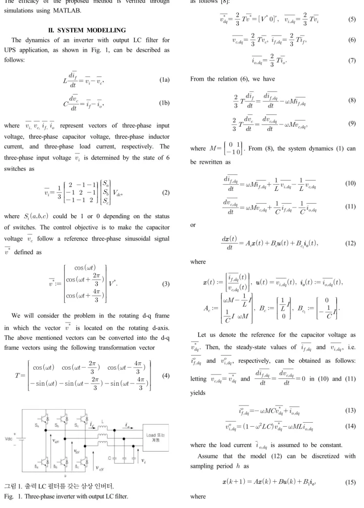
그림 1. 출력 LC 필터를 갖는 삼상 인버터.
Fig. 1. Three-phase inverter with output LC filter.
The efficacy of the proposed method is verified through simulations using MATLAB.
II. SYSTEM MODELLING
The dynamics of an inverter with output LC filter for UPS application, as shown in Fig. 1, can be described as follows:
, (1a)
, (1b)
where represent vectors of three-phase input voltage, three-phase capacitor voltage, three-phase inductor current, and three-phase load current, respectively. The three-phase input voltage is determined by the state of 6 switches as
, (2)
where could be 1 or 0 depending on the status of switches. The control objective is to make the capacitor voltage follow a reference three-phase sinusoidal signal
defined as
cos
cos
cos
(3)
We will consider the problem in the rotating d-q frame in which the vector is located on the rotating d-axis.
The above mentioned vectors can be converted into the d-q frame vectors using the following transformation vector
cos cos
cos
sin sin
sin
(4)
as follows [8]:
′
(5)
(6)
(7)
From the relation (6), we have
(8)
(9)
where
. From (8), the system dynamics (1) can be rewritten as
(10)
(11) or
(12)
where
Let us denote the reference for the capacitor voltage as
. Then, the steady-state values of and , i.e.
and , respectively, can be obtained as follows:
letting and
in (10) and (11) yields
(13)
(14)
where the load current is assumed to be constant.
Assume that the model (12) can be discretized with sampling period as
(15) where
U1
U2
U3
U4
U5
U6
O
ua b
2 2U t
1 1U t
Vdc
3 2 Vdc
3 2
a
b
그림 2. 스위칭함수의 공간벡터와 포화 입력제한.
Fig. 2. Space vector of the switching function and its saturation constraints.
The control input of (15) is implemented by using the space-vector PWM (SVPWM) method [11] after the
transform is applied. Given the set of three-phase switching functions as (2), the switching function space vector is defined as:
(16)
Since the switching functions s could be '0' or '1', then (16) can be rewritten in the generalized form for all switching states as
⋯
(17)
and the control input signal , which is the stationary frame (or -frame) representation of , can be generated as Fig. 2 using SVPWM. It is easy to see that the control input generated through the SVPWM method is constrained in the hexagon shown in Fig. 2. However, we consider a rather conservative, but simpler constraint that is the disk inscribed in the hexagon shown in Fig. 2. The disk-shaped constraint can also be stated in the rotating dq-frame as
′ ≤
. (18)
We will use the following control law based on the steady-state values of (13)-(14):
(19)
Inserting (19) into (15), we have
(20) Since the steady-state signals will satisfy
(21) subtracting (21) from (20) will give
(22) where
(23)
In the following section, we will develop a stabilizing control strategy for the discrete-time system (22) considering the input constraint (18).
III. FEASIBLE AND INVARIANT SETS
Many technologies developed in the previous works can be applied to define a feasible and invariant set for the system dynamics (22). [9,10] Consider the following ellipsoidal set:
′≤ ′ (24) The feasibility and invariance of the ellipsoidal set of (24) for the system (22) can be defined as follows:
Definition 1: Consider the system (22) with the steady-state values (13)-(14). The set (24) is feasible and invariant with respect to the feedback control if
satisfies the input constraint (18) for all ∈ (feasible) and the use of this control law guarantees
∈ for any ∈ (invariant).
Replacing with in (22), we have
(25)
where . From (25), we have
′ ′
′ ′ (26)
Thus, it is easy to see that
′ (27) guarantees the invariance of with respect to the control
. If we denote the distance between and the border of the hexagon (18) as , then
′ ≤ (28)
guarantees that satisfies the input constraint (18). Left and right multiplying of to
both sides of (27) yields
′ (29) where . Applying the Schur complement, (29) can be transformed into the following LMI:
′
(30) We need to lay additional constraints on so that the control of (19) satisfies the input constraint (28) for all ∈. Using and matrices, the condition (28) can be rewritten as
′ ′ ≤ (31)
A sufficient condition for all ∈ to satisfy (31) is
′ (32)
which can be transformed into the following LMI:
′
(33) Thus, a feasible and positively invariant set for the system (22) is defined by (24), (30) and (33).
The matrices and satisfying (30) and (33) would not be unique and we have some freedom in defining a criterion of selecting these matrices. The closed-loop stability of the control is stated as per the following theorem.
Theorem 1: Consider the system (22) with constraint (18). The state feedback control law
≥ guarantees that the Lyapunov value
′ will decreases monotonically for any initial state ∈, provided that the feedback gain and positive definite matrix are obtained by solving LMIs (30) and (33), where and .
Proof: The LMI (33) guarantees the feasibility of the
for any ∈ and (33) ensures (27) and the monotonicity of as (26). Note that this monotonicity implies the invariance of with respect to the control
. Thus, the feasibility of ≥
is guaranteed for any initial state ∈. ∎ It is clear that of Theorem 1 could be a Lyapunov function and the monotonicity of
guarantees the stability of the closed system. The choice of
(i.e. ) and satisfying (30) and (33) would determine the volume of and the performance of the control . Our preference is large volume of
and good performance but there is trade-off between them, i.e. large volume will result in loose control and tight control will result in small volume of .
In the following section, a novel method to combine a large invariant set with tight control will be derived.
IV. ON-LINE CONTROL ALGORITHM
We will combine a large feasible and invariant set with a degree of freedom to steer the error state well into the invariant set. In order to obtain a large volume of , consider the following optimization problem:
max tr (34) Maximizing the trace of will result in small and the volume of the corresponding ellipsoid will become large.
Solving the problem (34) will be done off-line. The on-line control strategy will be to use a degree of freedom to steer the current state deep into the ellipsoidal set , which can be done by solving the following problem for the given and the measured state :
min (35)
The solution of (35) can be obtained analytically. From (22), we have
′ ′ (36)
Thus, the unconstrained optimal solution of the problem (35) can be obtained from
as
′ ′ (37) Thus, the unconstrained optimal control is
(38) If this does not satisfy the input constraint (18), i.e.
is outside of the disk, then will take the minimum value at the point on the boundary of the disk. To obtain such point it is necessary to solve a nonlinear algebraic equation. An approximated solution can be found by searching along the boundary of the circle with the initial value given as
∥∥
⋅
. (39)
Thus, the overall algorithm can be summarized as follows:
1. IBCA (Invariance Based Control Algorithm) Off-line Procedure
- Obtain , and corresponding and by solving (34).
On-line Procedure (At each time step )
Step 1: Measure the load current and compute
the corresponding steady-state values and as (13)-(14) with given .
Step 2: Compute the unconstrained optimal solution
as (37) for the measured
Step 3: If given by (38) satisfies the input constraint, use it. Otherwise, search the constrained optimal control with the initial value (39) and use it.
The stability of the proposed Control Algorithm can be established as per the following Theorem.
Theorem 2: Consider the input constrained discrete-time system described by (15) and (18) with the steady state satisfying (21) for the measured value of and the control (19). The IBCA algorithm will guarantee that the error dynamics (22) become asymptotically stable, i.e. output voltage will be bounded and follow the reference signal asymptotically, provided that the output current
is constant and the initial error state belongs to the feasible and invariant set defined by the matrix of the Step 1 of IBCA algorithm.
Proof: From the feasible invariance of the with respect to the feedback gain , which is obtained in Step 1 of IBCA, the use of will guarantee the monotonic decrease of ′ for all
∈.
Since ∈ or is the constrained optimal solution of (35), the on-line procedure of IBCA searches a further reduction of than the use of .
Thus will remain in for all and will decrease to zero to yield the asymptotic stability of the
system (22). ∎
V. USE OF STATE/DISTURBANCE OBSERVER In the previous derivation, the capacitor voltage , inductor current , and load current are assumed to be measured. In many real applications, however, not both of
and is measured and it is required to estimate one of the currents. Furthermore, the steady-state condition (21) would not be satisfied in real plants because of the uncertainties in the plant parameters, measurements, and errors introduced in the discretization process. Hence, if the control law proposed in the last section is used, then there will be some offset error. To remove the offset error, PID controllers usually used [11,12]. We adopt, however, a disturbance observer to compensate all the uncertainties as in [4].
Under the assumption that the dynamics of the load current is much longer than the sampling time, the load current can be considered to be a constant signal. Thus, the
system (20) can be rewritten as follows with augmented states:
(40)
,
and , , and are defines in (20). The following Luenberger-type state estimator can be used for the system (40) for filtering or observing the states:
(41) where denotes the measured output and and are the estimated values of and , respectively. Depending on the employed measurements, is as follows:
a) and are measured : ′
b) and are measured : ′
In both cases, the measured output can be represented as
(42)
with proper matrix corresponding to the employed measurement. By inserting (42) and into (41), we have
(43)
VI. SIMULATION
The proposed control strategy was verified through simulation studies using MATLAB Simulink. The parameters of system (1) and (2) determined as L = 2.4 mH, C = 16 µF, and Vdc = 500 V. The reference voltage
of (3) was determined with = 220 V and it can be transformed into the reference voltage in d-q frame as the relation (5). Based on and the estimated output current , and are obtained as (13)-(14). The control gain was determined by solving problem (34) as
. The simulation time is 0.06 sec with 15 kHz sampling rate.
It was assumed that the inductor current and output voltage are measured. The gain of the state observer is chosen so that the observer poles are as follows:
The error is computed as (23) at each time step w.r.t. the steady-state values and as (13)-(14).
0 0.01 0.02 0.03 0.04 0.05 0.06 -6
-4 -2 0 2 4 6
0 0.01 0.02 0.03 0.04 0.05 0.06
-200 0 200
0 0.01 0.02 0.03 0.04 0.05 0.06
-4 -2 0 2 4
Time(sec)
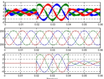
그림 3. 저항성부하에 대한 시뮬레이션: (상[A]), (중[ V]),
(하[ A]). 부하가 ∞, 50, 200 Ω으로 차례로 변함.
Fig. 3. Simulation results with resistive load: (upper: [A]), (middle: [V]) and (lower: [A]). The load changes as ∞, 50 and 200 Ω.
0 0.01 0.02 0.03 0.04 0.05 0.06
0 2 4
0 0.01 0.02 0.03 0.04 0.05 0.06
0 100 200
0 0.01 0.02 0.03 0.04 0.05 0.06
0 2 4
Time(sec)
그림 4. 저항성부하에 대한 시뮬레이션 dq축 표현: (상[A]),
(중[ V]), (하[ A]). 실선(점선)은 d축(q축) 값.
Fig. 4. Simulation results in d-q plane values with resistive load
(upper: [A]), (middle: [V]) and (lower: [A]);
Solid(dashed) lines represents the d-axis(q-axis) values.
0 0.01 0.02 0.03 0.04 0.05 0.06
-4 -2 0 2 4
0 0.01 0.02 0.03 0.04 0.05 0.06
-200 0 200
0 0.01 0.02 0.03 0.04 0.05 0.06
-4 -2 0 2 4
Time(sec)
그림 5. 정류기 부하에 대한 시뮬레이션 결과: (상[A]), (중[
V]), (하[ A]).
Fig. 5. Simulation results with rectifier load (upper: [A]), (middle: [V]) and (lower: [A]).
0 0.01 0.02 0.03 0.04 0.05 0.06
0 1 2 3
0 0.01 0.02 0.03 0.04 0.05 0.06
0 100 200 300
0 0.01 0.02 0.03 0.04 0.05 0.06
-1 0 1 2 3
Time(sec)
그림 6. 정류기 부하에 대한 시뮬레이션 결과 dq축 표현: (상 [A]), (중[ V]), (하[ A]). 실선(점선)은 d축(q축) 값.
Fig. 6. Simulation results in d-q plane values with rectifier load
(upper: [A]), (middle: [V]) and (lower: [A]);
Solid(dashed) lines represents the d-axis(q-axis) values.
Then we could make control input on d-q axis from (19).
The control input in d-q axis was changed to real switching input for three-phase IGBT Inverter by SVPWM [11]. The SVPWM switching frequency is 15 kHz to control three-phase inverter.
Fig. 3 shows the simulation result with resistive load.
The resistive load value is ∞ at 0 sec. We changed load values to 50 Ω at 0.02 sec and 200 Ω at 0.04 sec. Fig. 4 shows the same simulation results in d-q plane values. This simulation result shows the proposed control method can track the reference value very well. The voltage
THD(Total Harmonic Distortion) value is less than 1%.
Figs. 5 and 6 show simulation results with three-phase rectifier connected to 100 Ω resistor three-phase and d-q plane, respectively. The voltage THD(Total Harmonic Distortion) value is also less than 1 %.
VII. CONCLUSION
In this paper an efficient MPC method, based on the concept of invariant set, has been proposed for three-phase inverters with output LC filter. The control objective is to regulate the output voltage to a specified value using SVPWM technique.
In the off-line procedure, a large feasible and invariant set is derived. The on-line algorithm (ICBA) computes the optimal control input in the sense that the next state moves inside the invariant set as deep as possible. Unlike earlier works, ICBA provides a rigorous stability proof for the constrained system. The simulation examples have shown the good performance of the proposed ICBA.
In practice, a state estimator or filter is used as we have done in the simulation. However, the stability analysis of the closed-loop system combined with the estimator has not investigated and thus requires further study.
REFERENCES
[1] T. L. Tai and J. S. Chen, “UPS inverter design using discrete-time sliding-mode control scheme,” IEEE Trans.
Industrial Electronics, vol. 49, no. 1, pp. 67-75, Feb.
2002.
[2] O. Kuker, “Deadbeat control of a three-phase inverter with an output LC filter,” IEEE Trans. Power Electronics, vol. 11, no. 1, pp. 16-23, Jan. 1996.
[3] P. Mattavelli, “An improved deadbeat control for UPS using disturbance observer,” IEEE Trans. Industrial Electronics, vol. 52, no. 1, pp. 206-211, Feb. 2005.
[4] P. Cortes, G. Ortiz, J. I. Yuz, J. Rodriguez, S. Vazquez, and L. G. Franquelo, “Model predictive control of an inverter with output LC filter for UPS applications,”
IEEE Trans. on Industrial Electronics, vol. 56, no. 6, pp. 1875-1883, Jun. 2009.
[5] P. Cortes, J. Rodriguez, S. Vazquez, and L. G.
Franquelo, “Predictive control of a three-phase UPS inverter using two steps prediction horizon,” 2010 IEEE ICIT (International Conference on Industrial Technology), Vi a del Mar, pp. 1283-1288, Mar. 2010.
[6] P. C. Loh, M. J. Newman, D. N. Zmood, and D. G.
Holmes, “A comparative analysis of multiloop voltage regulation strategies for single and three-phase UPS systems,” IEEE Trans. on Power Electronics, vol. 18, no. 5, pp. 1176-1184, Sep. 2003.
[7] S. Boyd, L. E. Ghaoui, E. Feron, and V. Balakrishnan Linear Matrix Inequalities in System and Control Theory, SIAM, 1994.
[8] H. Komurcugil and O. Kuker, “Lyapunov-based control for three-phase PWM AC/DC voltage-source converters,”
IEEE Trans. on Power Electronics, vol. 13, no. 5, pp.
801-813, Sep. 1998.
[9] Y. I. Lee and B. Kouvaritakis, “Constrained robust
model predictive control based on periodic invariance,”
Automatica, vol. 42, no. 12, pp. 2175-2181, Dec. 2006.
[10] Y. I. Lee, B. Kouvaritakis, and M. Cannon, “Extended invariance and its use in model predictive control,”
Automatica, vol. 41, no. 12, pp. 2163-2169, Dec. 2005.
[11] M. H. Rashid, Power Electronics, 3rd Ed., Prentice-Hall, 2004.
[12] K.-P. Ahn, J.-S. Lee, J. S. Lim, and Y. I. Lee,
“Auto-tuning of PID/PIDA controllers based on step response,” Journal of Institute of Control, Robotics and Systems (in Korean), vol. 15, no. 10, pp. 974-981, Oct.
2009.
[13] M. S. Ali, J.-S. Lee, and Y. I. Lee, “Identification of three-parameter model from step response,” Journal of Institute of Control, Robotics and Systems (in Korean), vol. 16, no. 12, pp. 1189-1196, Dec. 2010.
임 재 식
1996년 경상대학교 제어계측공학과 졸
업. 2000년 동 대학원 석사. 2011년 서
울과학기술대학교 나노아이티공학과
박사. 현재 서울과학기술대학교 전기 정보기술연구소 연구원. 관심분야는 모델예측제어 이론과 전력변환기, 전 동기 제어에 모델예측제어 적용 등.
박 효 성
2006년~현재 서울과학기술대학교 제어
계측공학과 학부 재학. 관심분야는 컴 퓨터 프로그래밍 및 제어 이론 등.
이 영 일
1986년, 1988년, 1993년 서울대학교 제 어계측공학과 학사, 석사, 박사. 1994 년~2001년 7월 경상대학교 부교수.
2001년 8월~현재 서울과학기술대학교
제어계측공학과 교수. 1998년 2
월~1999년 7월 Dept. of Engineering science, Oxford University, Visiting research fellow. 2007년 9 월~2011.12 Editor of the International Journal of Control, Automatic, and system (IJCAS).