시각 인지 특성과 딥 컨볼루션 뉴럴 네트워크를 이용한 단일 영상 기반 HDR 영상 취득
비엔 지아 안a), 이 철a)‡
HVS-Aware Single-Shot HDR Imaging Using Deep Convolutional Neural Network
An Gia Viena) and Chul Leea)‡
요 약
본 논문은 딥 컨볼루션 뉴럴 네트워크(CNN)를 이용하여 행 별로 서로 다른 노출로 촬영된 단일 영상을 HDR 영상으로 변환하는 기법을 제안한다. 제안하는 알고리즘은 먼저 입력 영상에서 저조도 또는 포화로 인해 발생하는 정보 손실 영역을 CNN을 이용하여 복 원하여 휘도맵을 생성한다. 또한, CNN 학습 과정에서 인간의 시각 인지 특성을 고려할 수 있는 손실 함수를 제안한다. 마지막으로 복 원된 휘도맵에 디모자이킹 필터를 적용하여 최종 HDR 영상을 획득한다. 컴퓨터 모의실험을 통해 제안하는 알고리즘이 기존의 기법에 비해서 높은 품질의 HDR 영상을 취득하는 것을 확인한다.
Abstract
We propose a single-shot high dynamic range (HDR) imaging algorithm using a deep convolutional neural network (CNN) for row-wise varying exposures in a single image. The proposed algorithm restores missing information resulting from under- and/or over-exposed pixels in an input image and reconstructs the raw radiance map. The main contribution of this work is the development of a loss function for the CNN employing the human visual system (HVS) properties. Then, the HDR image is obtained by applying a demosaicing algorithm. Experimental results demonstrate that the proposed algorithm provides higher-quality HDR images than conventional algorithms.
Keyword : High dynamic range (HDR) imaging, spatially varying exposure (SVE) imaging, convolutional neural network (CNN)
Copyright Ⓒ 2016 Korean Institute of Broadcast and Media Engineers. All rights reserved.
“This is an Open-Access article distributed under the terms of the Creative Commons BY-NC-ND (http://creativecommons.org/licenses/by-nc-nd/3.0) which permits unrestricted non-commercial use, distribution, and reproduction in any medium, provided the original work is properly cited and not altered.”
a)부경대학교 컴퓨터공학과(Pukyong National University, Department of Computer Engineering)
‡Corresponding Author : 이철(Chul Lee)
E-mail: [email protected] Tel: +82-51-629-6228
ORCID: https://orcid.org/0000-0001-9329-7365
※이 논문은 부경대학교 자율창의학술연구비(2016년)에 의하여 연구되었음.
※This work was supported by a Research Grant of Pukyong National University (Year 2016).
・ Manuscript received March 22, 2018; Revised April 26, 2018; Accepted April 26, 2018.
특집논문 (Special Paper)
방송공학회논문지 제23권 제3호, 2018년 5월 (JBE Vol. 23, No. 3, May 2018) https://doi.org/10.5909/JBE.2018.23.3.369
ISSN 2287-9137 (Online) ISSN 1226-7953 (Print)
Ⅰ. Introduction
High dynamic range (HDR) imaging is a new imaging technique for representing pixel intensities in digital images and videos. The real world scenes contain richer in- formation than low dynamic range (LDR) images captured using conventional devices. Therefore, instead of using low range of intensities, e.g., 8-bits, an HDR image can repre- sent all intensity levels perceived by the human eye.
Because of its advantages over conventional imaging, many researches have been made for acquiring high-quality HDR images [1]. While a conventional camera’s sensor captures only a limited dynamic range of the scene, its dy- namic range can be extended by changing exposure times.
Hence, each image captured with different exposure time contains different information of the scene.
The conventional approach for HDR imaging is to cap- ture a stack of LDR images with different exposure times and merge them into a final HDR result [2]-[4]. However, this approach provides high performance only when the scene is static. If the scene contains moving objects or the camera is shaking while capturing images, the conventional approach fails to generate high-quality HDR results, yield- ing ghosting artifacts. To address such an issue, many HDR deghosting algorithms to remove ghosting artifacts have been proposed [5]-[9]. However, the main drawback of the conventional HDR deghosting algorithms is their high computational cost which limits the application of HDR imaging to practical applications.
An attempt to synthesize an HDR image that can avoid ghosting artifacts is to employ the spatially varying ex- posures (SVE) [10]. In an SVE-base algorithm, the scene is captured with pixel-wise varying exposures in a single image, and multiple subimages corresponding to each ex- posure are obtained. Then, the final HDR image is synthe- sized by merging the subimages. Because this approach provides high-quality HDR images without ghosting arti- facts, several algorithms have been recently developed to
improve the synthesis performance [10]-[16]. Most conven- tional single-shot HDR imaging algorithms recover the missing information in under- and/or over-exposure regions in an image from neighboring pixels of different exposure [11], [14]. However, these algorithms may provide artifacts and loss of sharp details caused by interpolation. Recently, An and Lee [17] proposed a deep learning-based approach to single-shot HDR imaging that recovers missing in- formation in under- and/or over-exposure regions. However, the reconstructed image still contains artifacts and noise.
This is because they employed the norm as a loss func- tion in training, which may fail to faithfully measure errors with extremely small or high values.
In this work, we propose a novel single-shot HDR imag- ing algorithm using a deep convolutional neural network (CNN). Specifically, we apply the CNN to reconstruct the radiance map of raw Bayer pattern image from an input SVE image. We develop a new loss function, which is in- spired by the human visual system (HVS) properties, to fill missing regions in the SVE raw Bayer image. Also, we an- alyze the effect of different loss functions, which are devel- oped for HDR imaging. Finally, we obtain the final HDR image by applying a demosaicing filter to the reconstructed radiance map. Experimental results show that the proposed algorithm provides higher quality HDR images than the state-of-the-art algorithms [11], [14], [17].
Ⅱ. Proposed Algorithm 1. Spatially Varying Exposure (SVE) Image
For SVE image acquisition, we employ the sensor archi- tecture in [11], [14], which uses a row-wise exposure encod- ing in a single raw Bayer image. Fig. 1 shows the Bayer pat- tern employed in this work. We consider the × RGGB Bayer color filter array with two different exposure times, i.e., short exposure time and long exposure time .
그림 1. 본 연구에서 적용한 컬러 필터 패턴
Fig. 1. Illustration of the Bayer pattern employed in this work
Specifically, the input image ∈ × is given by
= , on (4 + 1) and (4 + 2)th rows
, on (4 + 3) and (4 + 4)th rows (1)
where and denote the short and long exposure sub- images, respectively, and …
. In this work, we
assume that the bit-depth of the input image is an 8.
2. Radiance Map Reconstruction
We first convert the input SVE raw Bayer image to the irradiance map , assuming that the camera response function (CRF) is known a priori. Specifically, let denote the CRF [2], then the image acquisition is modeled as
(2)
where ∈ indexes the exposure time. Since the CRF
is invertible [2], the model in (2) can be rewritten as
ln ln (3)
where ln . Then, we can obtain the irradiance map
ln ln (4)
Since the input SVE raw Bayer image contains under- and/or over-exposed pixels, the irradiance map obtained by (4) includes unreliable irradiance values at the corre- sponding pixel locations as depicted by white color in Fig.
2. We recover those unreliable information in by using the CNN model developed in [17].
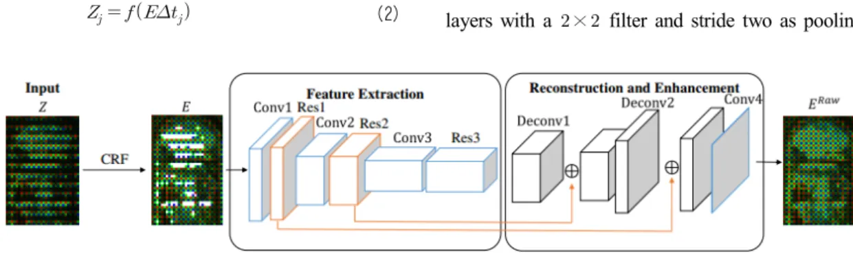
Fig. 2 shows the architecture of the CNN we use, which takes the irradiance map as input and reconstructs the radiance map . The network contains two stages. The first stage extracts the feature maps from the input image.
This contains three convolution layers (Conv1~Conv3) and three residual blocks (Res1~Res3) next to each convolution layer. The residual block contains two convolution layers and an identity mapping, which lets the network to learn an identify function in order to effectively fill missing val- ues in . We also apply the batch normalization [18] and ReLU activation function [19] to the output of each con- volution layer. Moreover, the network uses convolution layers with a × filter and stride two as pooling layers
그림 2. 입력 영상로부터 휘도맵를 복원하기 위한 CNN 구조 [17]
Fig. 2. The architecture of the CNN to reconstruct the raw Bayer radiance map from the input [17]
as done in [20] to reduce the spatial extent of feature maps while preserving spatial information. The second stage re- constructs the radiance map from the feature map and en- hances it. This stage contains two deconvolution layers (Deconv1 and Deconv2) and two skip connections. The de- convolution layers are convolution layers with fractional stride applied for the up-sampling. The skip connection is used to preserve the details and improve the final image quality by adding feature maps from Res1 and Res2 in the first stage to the corresponding Deconv1 and Deconv2 in the second stage.
3. Loss functions for radiance map reconstruction
In [17], the norm is used for the error function. Note that the norm penalizes larger errors, but it is more tol- erant to small errors regardless of the underlying structure in the image. Therefore, the norm is not a good choice for HDR imaging. As a result, An and Lee’s algorithm [17]
provides visible artifacts in the synthesized results. In this work, we compare the impact of different loss functions for HDR imaging. The loss function between the ground-truth images and the reconstructed images
can be formulated as
(5)
where denotes the error function, and is the number of batch training samples. Let us describe different error functions ∙ in (5) subsequently.
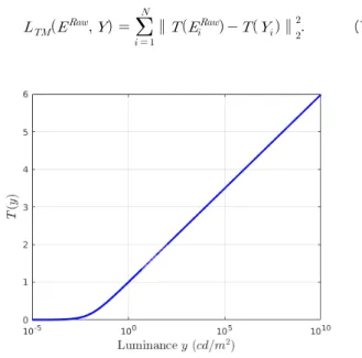
3.1 Norm Loss in Tone-mapped Image Domain The tone-mapping is the process to convert the HDR im- age to an LDR image. In [21], Kalantari and Ramamoorthi proposed to compute the loss function between HDR im- ages in the tone-mapped image domain. The tone-mapping models are generally complex and are differentiable.
Hence, they proposed to use the -law function as a tone-mapping function, which is given by
log
log
(6)
where is a parameter to control the degree of tone- mapping. In our experiment, we fix to 100. Fig. 3 illus- trates the tone-mapping function in (6). Then, the loss function between the estimated and the ground-truth images is defined as
∥ ∥ (7)
그림 3. 수식 (6)의 도시
Fig. 3. Illustration of the function in (6)
3.2 Illumination and Reflectance Loss Function As mentioned earlier, the norm loss function for- mulated directly on HDR values is significantly influenced by high luminance values, leading to the underestimation of important differences in the lower luminance ranges. To address such drawback, Eilertsen et al. [22] separated the HDR contents into two different components: the illumi- nance component and reflectance component . The illu- mination component contains the high luminance in- formation, while the reflectance component contains local
detail information. In order to obtain the illuminance com- ponent, they applied the Gaussian low-pass filter with ker- nel , where is the standard deviation. The re- flectance component is obtained by subtracting the illu- minance component from the input image. Then, the loss function is computed by the weighted average of the norms of the illuminance and reflectance components.
Specifically, the loss functions for and , respectively, are defined as
∥∗ log ∗ log ∥
(8)
where * denotes the convolution operator. Finally, the loss function is given by
(10)
where the parameter controls the relative importance be- tween the illuminance and reflectance components.
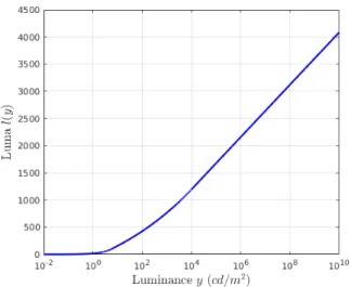
3.3 Human Visual System (HVS)-based Loss Function Note that the loss functions above are developed with less rigorous HVS models. Therefore, a synthesized HDR image with those loss function may provide perceptual differences with the ground-truth. In this work, we devel- op a loss function that is based on the more rigorous theo- retical human perceptual model [23]. Specifically, the lu- minance value given in is converted into percep- tually uniform integer values called luma, so that the error due to the rounding is not visible. For the HVS model, we employ the Blackwell’s model [24] to convert the lu- minance value to perceptually uniform luma value, which is defined as
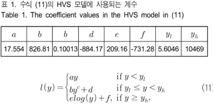
17.554 826.81 0.10013 -884.17 209.16 -731.28 5.6046 10469 표 1. 수식 (11)의 HVS 모델에 사용되는 계수
Table 1. The coefficient values in the HVS model in (11)
if
if ≤
if ≥ (11)
where the coefficients , , , , , , , and are listed in Table 1 [23]. Note that, because the HVS sensitivity var- ies with luminance levels, the conversion in (11) is com- posed of three different models to take account into such differences in sensitivity. Fig. 4 illustrates the lumi- nance-luma conversion in (11).
Then, we define the HVS-based loss function ∙
using the conversion in (11) as
∥ ∥. (12)
In the backpropagation, the backward function computes the partial derivative of the loss function in (12) with re- spect to each radiance value via
(13)
with
if
if ≤
if≥
(14)
∥log ∗ log log ∗ log ∥ (9)
그림 4. 수식 (11)의 luminance-luma 변환 도시
Fig. 4. Illustration of the luminance-luma conversion in (11)
4. Demosaicing
The reconstructed raw radiance map is mosaicked with the Bayer pattern (RGGB) as shown in Fig. 2. In or- der to obtain the final HDR image, we apply a demosaicing algorithm to recover the missing color values. In this work, we employ a simple image demosaicing algorithm based on the edge directed interpolation [25].
Ⅲ. Experimental Results
We evaluate the performance of the proposed single-shot HDR imaging algorithm both qualitatively and quantita- tively on ten HDR images, Apartment, BigfogMap, Dani_
Belgium, Dani_Cathedral, MemorialChurch, MPI_Atrium, MPI_Office, Nancy_Church, Nave, and SeymourPark.
However, due to the page limit, we only show the results only on two images in this paper. We compare the perform- ance of the proposed algorithm with those of Gu et al.’s algorithm [11], Cho et al.’s algorithm [14], and An and Lee’s algorithm [17]. We obtain the synthetic raw Bayer
images from the HDR image by sampling at each row to have ± f-stops, which corresponds to exposure times
and seconds, respectively. In addition, we trained the CNN network with a training set of 200,000 non- overlapping blocks of size × taken from 83 HDR im- ages1) of resolution × .
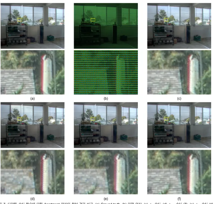
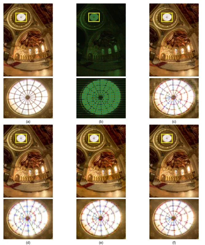
Figs. 5 and 6 show the synthesized results and their de- tailed parts on the Apartment and MemorialChurch image, respectively. Gu et al.’s algorithm [11] in Figs. 5(c) and 6(c), loses sharp details of the objects and yields artifacts in the synthesized images. For example, the blurring arti- facts and splotchy artifacts appear in Fig. 5(c) and Fig.
6(c), respectively. This is because their algorithm employs the bicubic interpolation to upsample the subimages and
to full the resolution. In Figs. 5(d) and 6(d), Cho et al.’s algorithm [14] outperforms Gu et al.’s algorithm, but it still provides artifacts, since their algorithm alleviates the line artifacts by apply the bilateral filtering-like inter- polation technique. For example, we can see the line arti- facts in Figs. 5(d) and 6(d). An and Lee’s algorithm [17]
synthesizes HDR images via CNN with the norm loss function. Figs. 5(e) and 6(e) shows that An and Lee’s algo- rithm provides higher synthesis results than Gu et al.’s and Cho et al.’s algorithms in term of color and details.
However, it still yields noise components around the edges due to the failure of loss function during training CNN. In contrast, the proposed algorithm in Figs. 5(f) and 6(f) pro- vides the best-quality results without visible artifacts, since the proposed HVS-based loss function effectively quanti- fies the loss in the CNN more faithfully than the loss function.
We compared three different loss functions in Section II-3. Figs. 7 and 8 show the synthesized results with those loss functions and their magnified parts on the Apartment and MemorialChurch image, respectively. The results of the loss function in Figs. 7(c) and 8(c) provide the noise
1) http://www.hdrlabs.com/sibl/archive.html
components around the edges. This indicates that the direct use of the loss function may fail in measuring the hu- manperception of image fidelity and quality. The results of the loss function, which uses the norm in the tone- mapped domain, contain severe artifacts in Figs. 7(d) and 8(d). Specifically, they contain color and splotchy artifacts in Fig. 7(d) and provides blurring artifact in Fig. 8(d).
While the results of the loss function in Figs. 7(e) and
8(e) provides higher qualities than the loss function, they still contain color artifacts and noise around the edges.
On the contrary, we can see that the proposed loss function yields higher quality HDR images without visible artifacts in Figs. 7(f) and 8(f).
In addition to the subjective evaluation, we compare the proposed algorithm with the conventional algorithms using three objective quality metrics: log-PSNR, perceptually
(a) (b) (c)
(d) (e) (f)
그림 5. Apartment 영상의 합성 결과 비교. (a) Ground-truth, (b) 입력 영상, (c) Gu 등의 알고리즘 [11], (d) Cho 등의 알고리즘 [14], (e) An 및 Lee의 알고리즘 [17], (f) 제안하는 기법
Fig. 5. Synthesized results of the Apartmentimage with different algorithms. (a) Ground-truth, (b) synthetic raw Bayer image, (c) Gu et al.’s algorithm [11], (d) Cho et al.’s algorithm [14], (e) An and Lee’s algorithm [17], and (f) the proposed algorithm
(a) (b) (c)
(d) (e) (f)
그림 6. MemorialChurch 영상의 합성 결과 비교. (a) Ground-truth, (b) 입력 영상, (c) Gu 등의 알고리즘 [11], (d) Cho 등의 알고리즘 [14], (e) An 및 Lee의 알고리즘 [17], (f) 제안하는 기법
Fig. 6. Synthesized results of the MemorialChurch image with different algorithms. (a) Ground truth, (b) synthetic raw Bayer image, (c) Gu et al.’s algorithm [11], (d) Cho et al.’s algorithm [14], (e) An and Lee’s algorithm [17], and (f) the proposed algorithm
uniform extension to PSNR (puPSNR) [26], high dynamic range visible difference predictor (HDR-VDP) [27]. The log-PSNR and puPSNR are extensions of the peak signal to noise (PSNR) by taking into account the model of the HVS to real-world luminance. HDR-VDP is a visual metric
that estimates the quality index score of the perceptual differences between the reference and the query images. A higher quality index score implies that the query image provides higher image quality with less differences com- pared to the reference.
(a) (b) (c)
(d) (e) (f)
그림 7. 다양한 손실 함수에 대한 Apartment 영상의 합성 결과 비교. (a) Ground-truth, (b) 입력 영상, (c) 손실, (d) 손실 (7), (e) 손실 (10), and (f) 손실 (12)
Fig. 7. Synthesized results of the Apartment image with different loss functions. (a) Ground-truth, (b) synthetic raw Bayer image, (c) loss, (d) loss in (7), (e) loss in (10), and (f) loss in (12)
(a) (b) (c)
(d) (e) (f)
그림 8. 다양한 손실 함수에 대한 Apartment 영상의 합성 결과 비교. (a) Ground-truth, (b) 입력 영상, (c) 손실, (d) 손실 (7), (e) 손실 (10), and (f) 손실 (12)
Fig. 8. Synthesized results of the MemorialChurch image with different loss functions. (a) Ground-truth, (b) synthetic raw Bayer image, (c) loss, (d) loss in (7), (e) loss in (10), and (f) loss in (12)
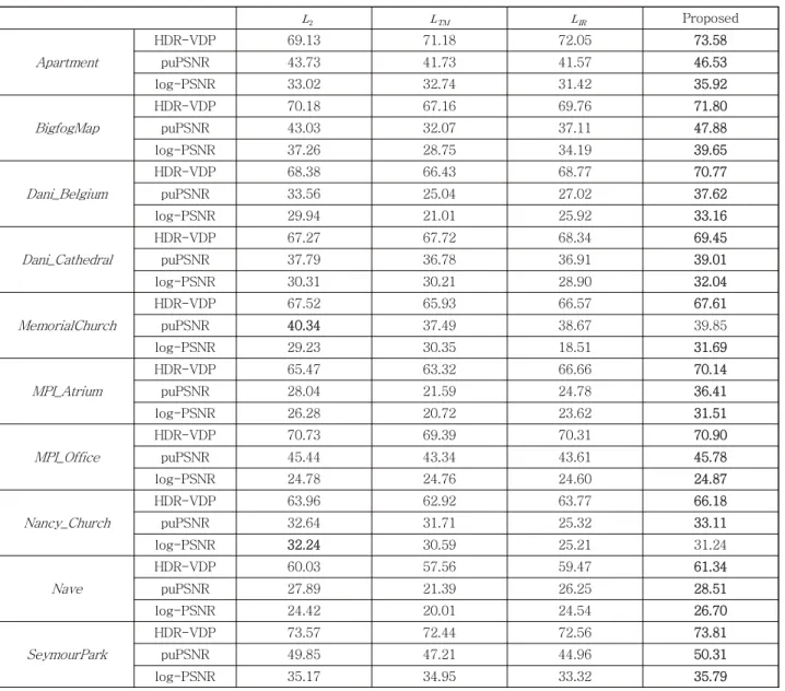
Table 2 quantitatively compares the reconstruction per- formance of the proposed algorithm with those of conven- tional algorithms over five images. Since the proposed al- gorithm efficiently considers the human perception model via the HVS-based loss function, it provides the best over-
all scores in term of all quality metrics. In addition, Table 3 lists the objective quality scores for different loss func- tion in the CNN. We can also see that the proposed HVS-model based loss provides the highest scores com- pared with conventional loss functions.
Gu et al. [11] Cho et al. [14] An and Lee [17] Proposed
Apartment
HDR-VDP 70.41 66.91 69.13 73.58
puPSNR 33.10 32.66 43.73 46.53
log-PSNR 28.29 28.59 33.02 35.92
BigfogMap
HDR-VDP 67.18 67.36 70.18 71.80
puPSNR 45.46 45.04 43.03 47.88
log-PSNR 36.67 37.59 37.26 39.65
Dani_Belgium
HDR-VDP 65.22 64.41 68.38 70.77
puPSNR 34.38 31.36 33.56 37.62
log-PSNR 29.81 27.47 29.94 33.16
Dani_Cathedral
HDR-VDP 65.97 66.91 67.27 69.45
puPSNR 32.74 33.44 37.79 39.01
log-PSNR 27.86 28.68 30.31 32.04
MemorialChurch
HDR-VDP 63.41 66.19 67.52 67.61
puPSNR 33.71 32.53 40.34 39.85
log-PSNR 26.79 27.23 29.23 31.69
MPI_Atrium
HDR-VDP 65.66 64.92 65.47 70.14
puPSNR 33.52 31.56 28.04 36.41
log-PSNR 26.28 28.19 26.28 31.51
MPI_Office
HDR-VDP 67.46 68.32 70.73 70.90
puPSNR 38.32 40.74 45.44 45.78
log-PSNR 25.61 35.63 24.78 24.87
Nancy_Church
HDR-VDP 60.50 65.24 63.96 66.18
puPSNR 27.14 25.75 32.64 33.11
log-PSNR 26.97 24.61 32.24 31.24
Nave
HDR-VDP 51.50 60.91 60.03 61.34
puPSNR 25.39 24.35 27.89 28.51
log-PSNR 24.41 22.54 24.42 26.70
SeymourPark
HDR-VDP 70.68 69.94 73.57 73.81
puPSNR 35.12 40.09 49.85 50.31
log-PSNR 29.49 32.46 35.17 35.79
표 2. puPSNR, log-PSNR, HDR-VDP를 이용한 HDR 영상 합성 성능의 정량적 비교
Table 2. Quantitative comparison of the HDR synthesis performance with different algorithms using puPSNR, log-PSNR, and HDR-VDP. The bold-face number denotes the best score
Ⅳ. Conclusions
We proposed a CNN-based single-shot HDR imaging al- gorithm in this work. We developed an HVS model-based loss function to quantify the visual differences between images. Then, we trained the CNN to recover unknown pixel values in under- and/or over-exposed regions in the
input image in the radiance domain. Experimental results demonstrated that the proposed algorithm outperforms the conventional algorithms in terms of both subjective and ob- jective qualities. In addition, we showed that the proposed HVS model-based loss function provides higher re- constructed performance than the conventional loss functions.
Proposed
Apartment
HDR-VDP 69.13 71.18 72.05 73.58
puPSNR 43.73 41.73 41.57 46.53
log-PSNR 33.02 32.74 31.42 35.92
BigfogMap
HDR-VDP 70.18 67.16 69.76 71.80
puPSNR 43.03 32.07 37.11 47.88
log-PSNR 37.26 28.75 34.19 39.65
Dani_Belgium
HDR-VDP 68.38 66.43 68.77 70.77
puPSNR 33.56 25.04 27.02 37.62
log-PSNR 29.94 21.01 25.92 33.16
Dani_Cathedral
HDR-VDP 67.27 67.72 68.34 69.45
puPSNR 37.79 36.78 36.91 39.01
log-PSNR 30.31 30.21 28.90 32.04
MemorialChurch
HDR-VDP 67.52 65.93 66.57 67.61
puPSNR 40.34 37.49 38.67 39.85
log-PSNR 29.23 30.35 18.51 31.69
MPI_Atrium
HDR-VDP 65.47 63.32 66.66 70.14
puPSNR 28.04 21.59 24.78 36.41
log-PSNR 26.28 20.72 23.62 31.51
MPI_Office
HDR-VDP 70.73 69.39 70.31 70.90
puPSNR 45.44 43.34 43.61 45.78
log-PSNR 24.78 24.76 24.60 24.87
Nancy_Church
HDR-VDP 63.96 62.92 63.77 66.18
puPSNR 32.64 31.71 25.32 33.11
log-PSNR 32.24 30.59 25.21 31.24
Nave
HDR-VDP 60.03 57.56 59.47 61.34
puPSNR 27.89 21.39 26.25 28.51
log-PSNR 24.42 20.01 24.54 26.70
SeymourPark
HDR-VDP 73.57 72.44 72.56 73.81
puPSNR 49.85 47.21 44.96 50.31
log-PSNR 35.17 34.95 33.32 35.79
표 3. puPSNR, log-PSNR, HDR-VDP를 이용한 다양한 손실 함수에 대한 HDR 영상 합성 성능의 정량적 비교
Table 3. Quantitative comparison of the HDR synthesis performance with different loss functions using puPSNR, log-PSNR, and HDR-VDP.
The bold-face number denotes the best score
참 고 문 헌 (References)
[1] P. Sen and C. Aguerrebere, “Practical High Dynamic Range Imaging of Everyday Scenes: Photographing The World as We Can See It with Our Own Eyes,” IEEE Signal Processing Magazine, Vol. 33, pp.
36-44, Sep. 2016.
[2] P. E. Debevec and J. Malik, “Recovering High Dynamic Range Radiance Maps from Photographs,” Proceeding of ACM SIGGRAPH, Aug. pp. 369-378, 1997.
[3] T. Mitsunaga and S. K. Nayar, “Radiometric Self-Calibration,”
Proceeding of IEEE Conference on Computer Vision and Pattern Recognition, pp.374-380, Jun. 1999.
[4] M. Aggarwal and N. Ahuja, “Split Aperture Imaging for High Dynamic Range,” Proceeding of IEEE International Conference on Computer Vision, Vol. 2, pp. 10-17, Jul. 2001.
[5] H. Zimmer, A. Bruhn, and J. Weickert, “Freehand HDR Imaging of Moving Scenes with Simultaneous Resolution Enhancement,”
Computer Graphics Forum, Vol. 30, pp. 405-414, Apr. 2011.
[6] P. Sen, N. K. Kalantari, M. Yaesoubi, S. Darabi, D. B. Goldman, and E.
Shechtman, “Robust Patch-Based HDR Reconstruction of Dynamic Scenes,” ACM Transactions on Graphics, Vol. 31, No. 6, pp.
203:1-203:11, Nov. 2012.
[7] C. Lee, Y. Li, and V. Monga, “Ghost-free High Dynamic Range Imaging via Rank Minimization,” IEEE Signal Processing Letters, Vol. 21, No.9, pp. 1045-1049, Sep. 2014.
[8] Y. Li, C. Lee, and V. Monga, “A Maximum a Posteriori Estimation Framework for Robust High Dynamic Range Video Synthesis,” IEEE Transactions on Image Processing, Vol. 26, No. 3, pp. 1143-1157, Mar. 2017.
[9] C. Lee and E. Y. Lam, “Computationally Efficient Truncated Nuclear Norm Minimization for High Dynamic Range Imaging,” IEEE Transactions on Image Processing, Vol. 25, No. 9, pp. 4145-4157, Sep. 2016.
[10] S. K. Nayar and T. Mitsunaga, “High Dynamic Range Imaging:
Spatially Varying Pixel Exposures,” Proceeding of IEEE Conference on Computer Vision and Pattern Recognition, Vol. 1, pp. 472-479, Jun.
2000.
[11] J. Gu, Y. Hitomi, T. Mitsunaga, and S. Nayar, “Coded Rolling Shutter Photography: Flexible Space-Time Sampling,” Proceeding of IEEE International Conference on Computational Photography, pp. 1-8, Mar. 2010.
[12] K. Hirakawa and P. M. Simon, “Single-Shot High Dynamic Range Imaging with Conventional Camera Hardware,” Proceeding of IEEE International Conference on Computer Vision, pp. 1339-1346, Nov.
2011.
[13] C. Aguerrebere, A. Almansa, Y. Gousseau, J. Delon, and P. Muse,
“Single Shot High Dynamic Range Imaging Using Piecewise Linear
Estimators,” Proceeding of IEEE International Conference on Computational Photography, pp. 1-10, May 2014.
[14] H. Cho, S. J. Kim, and S. Lee, “Single-Shot High Dynamic Range Imaging Using Coded Electronic Shutter,” Computer Graphics Forum, Vol. 33, No. 7, pp. 329-338, Oct. 2014.
[15] A. Serrano, F. Heide, D. Gutierrez, G. Wetzstein, and B. Masia,
“Convolutional Sparse Coding for High Dynamic Range Imaging,”
Computer Graphics Forum, Vol. 35, No. 2, pp. 153-163, May 2016.
[16] J. Li, C. Bai, Z. Lin, and J. Yun, “Penrose High-Dynamic-Range Imaging,” Journal of Electronic Imaging, Vol. 25, No. 3, pp. 033 024:1-13, Jun. 2016.
[17] V. G. An and C. Lee, “Single-Shot High Dynamic Range Imaging via Deep Convolutional Neural Network,” Proceeding of APSIPA ASC, pp. 1768-1772, Dec. 2017.
[18] S. Ioffe and C. Szegedy, “Batch Normalization: Accelerating Deep Network Training by Reducing Internal Covariate Shift,” Proceeding of International Conference on Machine Learning, pp. 448-456, Jul.
2015.
[19] V. Nair and G. E. Hilton, “Rectified Linear Units Improve Restricted Boltzman Machines,” Proceeding of International Conference on Machine Learning, pp. 807-814, Jun. 2010.
[20] J. Johson, A. Alahi, and F. F. Li, “Perceptual Losses for Real-Time Style Transfer and Super-Resolution,” Proceeding of European Conference on Computer Vision, pp. 694-711, Oct. 2016.
[21] N. K. Kalantari and R. Ramamoorthi, “Deep High Dynamic Range Imaging of Dynamic Scenes,” ACM Transactions on Graphics, Vol.
36, No. 4, Jul. 2017.
[22] G. Eilertsen, J. Kronander, G. Denes, R. K. Mantiuk, and J. Unger,
“HDR Image Reconstruction from a Single Exposure Using Deep CNNs,” ACM Transactions on Graphics, Vol. 36, No. 6, Nov. 2017.
[23] R. Mantiuk, K. Myszkowski, and H. P. Seidel, “Lossy Compression of High Dynamic Range Images and Video,” Proceeding of SPIE, Vol.
6057, Feb. 2006.
[24] O. Blackwell and H. Blackwell, “Visual Performance Data for 156 Normal Observers of Various Ages,” Journal of the Illuminating Engineering Society, Vol. 1, No. 1, pp. 3-13, 1971.
[25] J. E. Adams, “Design of Practical Color Filter Array Interpolation Algorithms for Digital Cameras,” Proceeding of SPIE, Vol. 3028, pp.
117-125, Feb. 1997.
[26] T. O. Aydin, R. Mantiuk, and H. P. Seidel, “Extending Quality Metrics to Full Luminance Range Images,” Proceeding of SPIE, Vol. 6806, p.
68060B, Mar. 2008.
[27] M. Narwaria, R. K. Mantiuk, M. P. D. Silva, and P. L. Callet,
“HDR-VDP-2.2: A Calibrated Method for Objective Quality Prediction of High Dynamic Range and Standard Images,” Journal of Electronic Imaging, Vol. 24, No. 1, Jan. 2015.
저 자 소 개
비엔 지아 안
- 2015년 : University of Science, Vietnam, Bachelor of Computer Science - 2016년 ~ 현재 : 부경대학교 컴퓨터공학과 석사과정
- ORCID : https://orcid.org/0000-0003-0067-0285 - 주관심분야 : 계산사진학, 영상처리, 컴퓨터비전
이 철
- 2003년 : 고려대학교 전기전자전파공학부 공학사 - 2008년 : 고려대학교 전자전기공학과 공학석사 - 2013년 : 고려대학교 전자전기공학과 공학박사 - 2002년 ~ 2006년 : ㈜바이오스페이스 (현 ㈜인바디)
- 2013년 ~ 2014년 : Postdoctoral Scholar, Pennsylvania State University - 2014년 ~ 2015년 : Research Scientist, The University of Hong Kong - 2015년 ∼ 현재 : 부경대학교 컴퓨터공학과 조교수
- ORCID : https://orcid.org/0000-0001-9329-7365 - 주관심분야 : 영상처리, 계산사진학, 컴퓨터비전
![그림 5. Apartment 영상의 합성 결과 비교. (a) Ground-truth, (b) 입력 영상, (c) Gu 등의 알고리즘 [11], (d) Cho 등의 알고리즘 [14], (e) An 및 Lee의 알고리즘 [17], (f) 제안하는 기법](https://thumb-ap.123doks.com/thumbv2/123dokinfo/4788785.520193/7.892.110.787.168.809/apartment-영상의-ground-알고리즘-알고리즘-lee의-알고리즘-제안하는.webp)
![그림 6. MemorialChurch 영상의 합성 결과 비교. (a) Ground-truth, (b) 입력 영상, (c) Gu 등의 알고리즘 [11], (d) Cho 등의 알고리즘 [14], (e) An 및 Lee 의 알고리즘 [17], (f) 제안하는 기법](https://thumb-ap.123doks.com/thumbv2/123dokinfo/4788785.520193/8.892.113.777.175.979/그림-memorialchurch-영상의-ground-알고리즘-알고리즘-알고리즘-제안하는.webp)