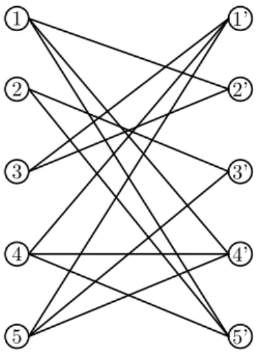
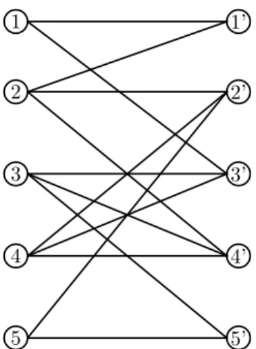
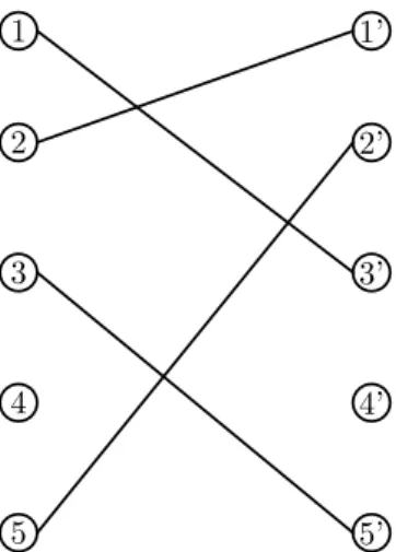
Graph representations of normal matrices
10
0
0
전체 글
(2)
(3)
(4)
(5)
(6)
(7)
(8)
(9)
(10)
수치

관련 문서
Nail clipper CD player Vending machine Nail clipper, CD player, Vending machine Mechanical engineering is a field of making a g g g. useful mechanism or machine by using
Gray and black vertices, therefore, have been discovered, but breadth-first search distinguishes between them to ensure that the search proceeds in a breadth-first manner..
• Solution 1: Break diffusion area by gaps (find a set of trails covering the graph). --> Minimize number of gaps (minimize
• Euler’s formula gives a relation among numbers of faces, vertices, and edges of a crossing-free drawing of a planar graph. n=9 vertices m=12 edges m=12
Calculate the magnitudes of the shear force, bending moment, and torsional moment acting g g on a transverse section through the frame at point O, located at some distance
Consider the motion of a particle of mass m which is constrained to move on the surface of a cone of half-angle α and which is subject to a gravitational force g. Let the
How to tackle: large graphs, online setting, graph construction …. One example: Online
Discuss the machine learning background of auto-regressive model to obtain the
