ON-BOARD REALTIME ORBIT PARAMETER GENERATOR FOR GEOSTATIONARY SATELLITE
Bong-Kyu Park, Koon-Ho Yang
COMS Program Office, KARI, [email protected]
ABSTRACT ... This paper proposes an on-board orbit data generation algorithm for geostationary satellites. The concept of the proposed algorithm is as follows. From the ground, the position and velocity deviations with respect to the assumed reference orbit are computed for 48 hours of time duration in 30 minutes interval, and the generated data are up-loaded to the satellite to be stored. From the table, three nearest data sets are selected to compute position and velocity deviation for the asked epoch time by applying 2nd order polynomial interpolation. The computed position and velocity deviations are added to reference orbit to recover absolute orbit information. Here, the reference orbit is selected to be ideal geostationary orbit with a zero inclination and zero eccentricity. Thanks to very low computational burden, this algorithm allows us to generate orbit data at 1Hz or even higher. In order to support 48 hours autonomy, maximum 3K byte memory is required as orbit data storage. It is estimated that this additional memory requirement is acceptable for geostationary satellite application.
KEY WORDS: Geostationary Satellite, Observation Satellite, On-board Orbit Propagator
1. INTRODUCTION
Geostationary observatory satellites like COMS (Communication, Ocean and Meteorological Satellite) heavily depend on the ground based post processing in order to provide high quality images. The land mark matching technique is a typical example of ground based image processing.(Ju etal.,2007) ABI system which is under development by ITT for next geostationary meteorological satellites provides very high rate of image samplings. In order to benefit from new capacity of high rate image samplings and to disseminate image data in real-time, we need to reduce the ground based post processing as much as possible, which in turn requires acquisition of raw image data as higher quality as possible. In consequence, very accurate satellite attitude and orbit information are required to compensate attitude and orbit errors. In case of ABI, the orbit data in following accuracy are asked in 1 Hz sampling rate.(Ellis etal., 2008)
•Satellite position error:
-35 m in-track -35 m cross-track -70 m radial/15 minutes
•Satellite velocity error:
-less than 6 cm/sec uncertainty per axis
It is not easy to meet this requirement in 1 Hz sampling rate. To begin with, as a solution, we can think about a system providing the orbit data from the ground system after orbit determination. But this system is not stable
enough because of possible failure of ground software and loss of RF-link.
It is recommended to install on-board orbit generator to make the system stable and autonomous for certain time of duration. Concerning the autonomy of the system, the COMS requires 48 hours autonomy. This system can be divided into two parts; the orbit determination part and the orbit prediction part. For orbit determination, the ranging data should be collected by the satellite. For LEO(Low Earth Orbit) satellite, the GPS signal can be used for this purpose as introduced by Jung etal(2003).
But for geostationary satellites which are positioned at higher altitude than GPS, it is not easy to receive GPS signal and related technologies are premature. It is difficult to implement on-board orbit determination system for geostationary satellite. Therefore, the ranging and orbit determination system shall be placed on the ground.
Concerning the on-board orbit propagator, it shall be very simple for low computational burden as heritage satellite system does not provide powerful computing environment. Jung etal(2003) proposed on-board orbit propagator based on GPS and residual reconstruction function for LEO satellite. But according to the analysis results, the accuracy does not meet the requirement of ABI system and the system is for LEO satellite.
Taking in to account the previously mentioned problems, this paper proposes a new on-board orbit parameter generation algorithm which is very simple and practical. From the ground, the position and velocity deviations with respect to the assumed reference orbit are computed for given time duration in 30 minutes interval, and the generated data are up-loaded to the satellite.
From the table, three nearest data sets are selected to compute position and velocity deviation for asked epoch time by applying 2nd order polynomial interpolation. The computed position and velocity deviation data are added to reference orbit to recover absolute orbit information.
Here, the reference orbit can be assumed to be an ideal geostationary orbit with a zero inclination and zero eccentricity.
2. ON-BOARD ORBIT PARAMETER GENERATION ALGORITHM
2.1 Equations
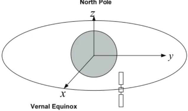
In this paper, the equations are described in ECI coordinate shown in Figure 1.(Pocha, 1987) The x-axis points the vernal equinox, the z-axis aheads the north pole and y-axis is selected in a way to complete the right- handed coordinate.
x
y
z
Figure 1. Earth Centered Inertial Coordinate The position of the satellite can be divided into two components: the reference and deviations from the reference, as shown in Figure 2. Here the reference can be selected to be a circular orbit with zero inclination.
x
y
z
θr Rr R
δR
Figure 2. Reference and Real Orbit
In this case, the position can be described as follows;
δR R
R= r + (1)
[ x y z ]
T=
R
(2)⎥⎥
⎥
⎦
⎤
⎢⎢
⎢
⎣
⎡
− +
− +
=
⎥⎥
⎥
⎦
⎤
⎢⎢
⎢
⎣
⎡
=
0
)]
( sin[
)]
( cos[
o o
o o
t t
t t R
z y x
e e s
r r r
ω θ
ω θ
Rr (3)
Here Rs means the distance of the geostationary satellite from the earth center, and its approximated value
is 42,164km. The ωe is the spin rate of the earth which is 7.2921157e-5 rad/sec.
Same principal can be applied for the description of the satellite velocity as follows;
δV V
V= r + (4)
[
x& y& z&]
T=
V (5)
⎥⎥
⎥
⎦
⎤
⎢⎢
⎢
⎣
⎡
− +
− +
−
=
⎥⎥
⎥
⎦
⎤
⎢⎢
⎢
⎣
⎡
=
0
)]
( cos[
)]
( sin[
o o
o o
&
&
&
t t
t t V
z y x
e e s
r r r
ω θ
ω θ
Vr (6)
Here, Vs means the velocity of the geostationary satellite and it can be simply computed as follows;
074648 .
=3
= s e
s R
V ω (7)
From the equations from (1) to (7), we can find that the orbit can be described by a simple reference orbit and deviation from the reference orbit.
2.2 Ground Data Preparation
As previously described, the ground system performs orbit determination and orbit prediction, and computers difference between the obtained orbit and the reference orbit in order to compute deviation from the reference orbit.
Rr
R
δR= − (8)
Vr
V
δV= − (9) Following seven parameters are uploaded to the satellites in given time interval; for example in 30 minutes time interval.
[ ]
ik t x y z x y z
X = δ δ δ δ& δ& δ& (10) If we assume that each parameter is stored in 4 byte data type and the time interval is 30 minutes, the total required memory size can be computed approximately to be 2,688 bytes. According to our experience, it is understood that 2,688 bytes is acceptable for COMS heritage.
2.3 On-Board Data Processing
On-board flight software can compute orbit data in 1Hz or even higher frequency by interpolating uploaded deviation data. For the interpolation based on 2nd order polynomial, Xk,Xk+1,XK=2, 3 nearest data to given epoch time are selected. And from following equations, we can obtain xi(t), the components of Xt.
i i i
i t at bt c
x ( )= 2+ + , i=1,...,6 (11)
⎥⎥
⎥
⎦
⎤
⎢⎢
⎢
⎣
⎡
⎥⎥
⎥
⎦
⎤
⎢⎢
⎢
⎣
⎡
=
⎥⎥
⎥
⎦
⎤
⎢⎢
⎢
⎣
⎡
+ +
−
+ +
+ +
) (
) (
) ( 1
1 1
2 1 1
2 2
2 1 2
1 2
k i
k i
k i
k k
k k
k k
i i i
t x
t x
t x t
t t t
t t c b a
(12)
⎥⎥
⎥
⎦
⎤
⎢⎢
⎢
⎣
⎡
− +
−
−
+
−
− +
−
− +
−
−
=
⎥⎥
⎥
⎦
⎤
⎢⎢
⎢
⎣
⎡
+ + + +
+ + +
+
+ + + + + + + +
−
+ +
+ +
2 1 1 2 2
1 2 1
2 2 2 2 2
2 2 2
2 2 1 2 2
1 2
2 2
1 2 1 1
2 2
2 1 2
1 2
1 1 1
k k k k k k k k
k k k k k k k k
k k k k k k k k
k k
k k
k k
t t t t t t t t
t t t t t
t t t
t t t t t t t t C t
t t t
t t
(13)
2 2 2
1 1 2
2 2
2 2 2
1 1 2
1
+ +
+ + + + +
+ + + − − −
=
k k k k k k k k k k k
kt t t t t t t t t t t
C t (14)
Equations from (11) to (14) shall be repeatedly applied for the computations of the 6 orbit parameters. However, as the values from equation (13) and (14) are same for all 6 parameters for given time, single computation is enough for the 6 parameters. Hence, only small computational burden are additionally asked for orbit parameter computation.
3. SIMULATION AND DISCUSSION
In order to estimate the performance of proposed algorithm, simulations have been performed for the following three cases.
CASE I: Linear interpolation using 30 minutes time interval data
CASE II: Interpolation using 2nd order polynomial and 30 minutes time interval
CASE III: Interpolation using 2nd order polynomial and 60 minutes time interval
In this simulation, 48 hours autonomy has been considered. And it has been assumed that the nominal longitude of the satellite is 128 deg.E. Figure 3 and 4 show the resulted position and velocity deviations from the reference orbit.
-50 -25 0 25 50
0 10 20 30 40 50
Rz Ry Rx
Elapsed Time(Hours)
Deviation(Km)
Figure 3. Position Deviation from Reference Orbit
-0.003 -0.001 0.001 0.003
0 10 20 30 40 50
Vz Vy Vx
Elapsed Time(Hours)
Deviation Velocity(Km/sec)
Figure 4. Velocity Deviation from Reference Orbit
3.1 Linear Interpolation
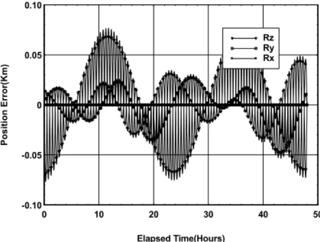
Figure 5 and 6 show the position and velocity errors for the final product under assumption of using the linear interpolation for 30 minutes data time interval. In case of position, the error in z-component nearly reaches up to 80 meters. This means that by the linear interpolation, we can not meet requirements. But in case of velocity, the error remains under 1cm/sec. and meets requirements. In consequence, using linear interpolation is not a good idea for orbit data recovery for ABI purpose.
3.2 Interpolation using 2nd Order Polynomial
Figure 7 and 8 show the position and velocity errors for the final product when 2nd order polynomial interpolation and 30 minutes data time interval have been assumed. In case of position error, it remains under 6 meters level for 48 hours. And for velocity error, its maximum value is under 0.8mm/sec. Therefore, we can conclude that when we use an interpolation based on 2nd order polynomial and 30 minutes interval orbit data, it is possible to meet the requirement given by ABI system with sufficient margin. Here, the position and velocity error means the deviation of the recovered orbit from the simulated orbit after orbit determination. Therefore, the difference between recovered orbit data and real orbit data heavily depends on accuracy of orbit determination error. In order to keep the error in small range, an accurate orbit determination technique shall be applied.
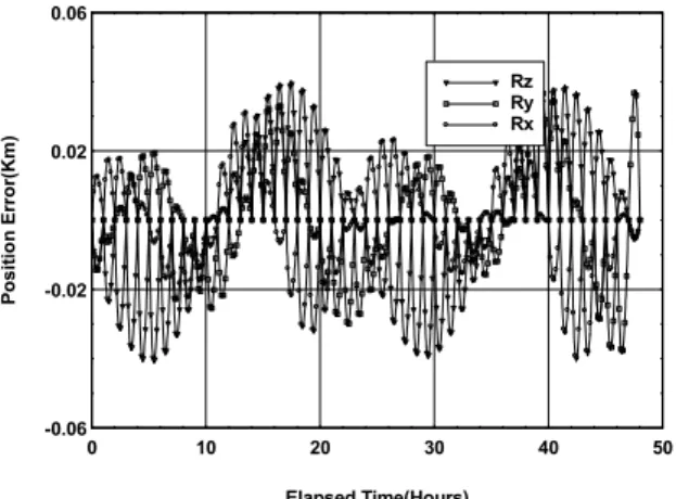
3.3 Interpolation using Data in 1hour Interval If the time interval can be extended from 30 minutes to some hours, we can reduce memory size required. In order to analyze the possibility of extension of time interval, a simulation has been performed under assumption of 1 hour time interval. Figure 9 shows the resulted position errors. Unfortunately, it is found that the x and z-axis error components grow up to 40 meters level which does not meet 35 meter requirement given by ABI system. By this simulation, we can conclude that 30 minutes time interval is a good selection for this system.
-0.10 -0.05 0 0.05 0.10
0 10 20 30 40 50
Rz Ry Rx
Elapsed Time(Hours)
Position Error(Km)
Figure 5. Position Error(Linear Interpolation)
-0.75 -0.25 0.25 0.75
0 10 20 30 40 50
Vz Vy Vx
Elapsed Time(Hours)
Velocity Error(cm/sec)
Figure 6. Velocity Error(Linear Interpolation)
-0.006 -0.002 0.002 0.006
0 10 20 30 40 50
Rz Ry Rx
Elapsed Time(Hours)
Position Error(Km)
Figure 7. Position Error(2nd Order Polynomial)
-0.08 -0.04 0 0.04 0.08
0 10 20 30 40 50
Vz Vy Vx
Elapsed Time(Hours)
Velocity Error(cm/sec)
Figure 8. Velocity Error(2nd Order Polynomial)
-0.06 -0.02 0.02 0.06
0 10 20 30 40 50
Rz Ry Rx
Elapsed Time(Hours)
Position Error(Km)
Figure 9. Position Error(1hour Interval, 2nd Order Polynomial)
4. CONCLUSIONS
This paper proposes a practical on-board orbit parameter generator for geostationary observatory satellites. The simulation results show that interpolation based on 2nd order polynomial and deviation data from the reference orbit in 30 minutes interval can recover orbit data with accuracy of 10 meter in position and 0.8mm/sec in velocity. This result meets the accuracy requirement for ABI system with sufficient margin.
Additional memory size for implementation of proposed system is around 3Kbyte which is acceptable in COMS heritage.
It has been concluded from the simulations that using linear interpolation or 1 hour interval data is not proper in term of accuracy.
REFERENCES
Gwang Hyeok Ju, Young Woong Park, Koon Ho Yang, INR(Image Navigation & Registration) System for COMS(Communication, Ocean, Meteorological Satellite, KSAS 2007 Fall Conference.
Ken Ellis, David Igli, Krishnaswamy Gounder, Paul Griffith, James Ogle, Vincent Virgilio, 2008. GOES-R Advanced Baseline Imager Image and Registration, 5th GOES Users' Conference.
Ok Chul Jung, Tae Soo No, Sang Ryool Lee, 2003. A study on Autonomous Update of Onboard Orbit Propagator, Journal of The Korean Society Aeronautical and Space Sciences Vol. 31No. 9, pp.51-59.
Pocha, J.J., 1987. Mission Design For Geostationary Satellites, Space Technology Library.