Fault Diagnosis System based on Sound using Feature Extraction Method of Frequency Domain

1. INTRODUCTION

Machine fault diagnosis (MFD) is the process of analyzing and understanding the signals gen- erated by the machines in order to detect whether they work in a normal or abnormal state. For its capacity of preventing accidents in the industry sites and avoiding sudden breakdowns in the pro- duction line, MFD is more than necessary for the

good performance of the industrial companies.

MFD schemes are based on the detailed analysis of the signals, like vibration or sound, which can be generated by the machines under inspection.

Unfortunately, those signals are usually disturbed and corrupted by unwanted noises from the envi- ronment that make the analysis to be a real chal- lenging task. Therefore, machine fault diagnosis systems are systematically thought as pattern rec-

Fault Diagnosis System based on Sound using Feature Extraction Method of Frequency Domain

Caleb Vununu^†, Oh-Heum Kwon^††, Kwang-Seok Moon^†††, Suk-Hwan Lee^††††, Ki-Ryong Kwon^{†††††}

ABSTRACT

Sound based machine fault diagnosis is the process consisting of detecting automatically the damages that affect the machines by analyzing the sounds they produce during their operating time. The collected sounds being inevitably corrupted by random disturbance, the most important part of the diagnosis consists of discovering the hidden elements inside the data that can reveal the faulty patterns. This paper presents a novel feature extraction methodology that combines various digital signal processing and pattern recognition methods for the analysis of the sounds produced by the drills. Using the Fourier analysis, the magnitude spectrum of the sounds are extracted, converted into two-dimensional vectors and uniformly normalized in such a way that they can be represented as 8-bit grayscale images. Histogram equalization is then performed over the obtained images in order to adjust their very poor contrast. The obtained contrast enhanced images will be used as the features of our diagnosis system. Finally, principal component analysis is performed over the image features for reducing their dimensions and a nonlinear classifier is adopted to produce the final response. Unlike the conventional features, the results demonstrate that the proposed feature extraction method manages to capture the hidden health patterns of the sound.

Key words: Pattern Recognition, Machine Learning, Machine Fault Diagnosis, Magnitude Spectrum, Principal Component Analysis, Artificial Neural Network

※ Corresponding Author : Ki-Ryong Kwon, Address:

(48513) 45 Yongso-ro, Namgu, Busan, Pukyong National University, Korea, TEL : +82-51-629-6257, FAX : +82-51-629-6230, E-mail : [email protected] Receipt date : Jan. 29, 2018 , Revision date : Mar. 22, 2018 Approval date : Mar. 28, 2018

††Dept. of IT Convergence and Application Engineering, Pukyong National University

(E-mail : [email protected])

††Dept. of IT Convergence and Application Engineering, Pukyong National University

(E-mail : [email protected])

†††††Dept. of Electronics Engineering, Pukyong National University (E-mail : [email protected])

†††††Dept. of Information Security, Tongmyong University (E-mail : [email protected])

†††††Dept. of IT Convergence and Application Engineering, Pukyong National University

※ This research was supported by Basic Science Re- search Program through the National Research Foundation of Korea(NRF) funded by the Ministry of Science and ICT(No. 2016R1D1A3B03931003, No. 2017R1A2B2012456) and he Korea Technology and Information Promotion Agency for SMEs(TIPA) grant funded by the Korea government(Ministry of SMEs and Startups) (No. C0407372).

ognition tasks [1-5].

Pattern recognition methodology consists of three steps: data acquisition, feature extraction and the final diagnosis based on a discrimination anal- ysis of the data. Data acquisition is the process of collecting the signals that will be used for the analysis. Sound data [6] have proven their capa- bility of carrying the operating states of the machines. In this work, we use the sounds gen- erated by the drills during their active time in the industry site, while the targeted damage consists of the wear that consumes the bit of the drills.

Feature extraction is the process of finding the best possible representation of the acquired data (vibration or sounds) in order to discover the ma- chine’s state patterns located inside them. Because the noises really affect their nature, the collected data do not expose their internal characteristics at first sight, being highly correlated between them and very much redundant. Using them without any significant transformation can pose huge problems not only in terms of the assessment’s accuracy but also in terms of the processing time. Thus, the pat- tern recognition methodology requires a feature extraction step where a short and precise version of the originally acquired data is created using dif- ferent kinds of methods. In fact, all the MFD sys- tems try to present a feature extraction method- ology that maximizes the accuracy of the final step, which makes the feature extraction to be the most important step of the MFD systems. We under- stand that a good feature selection method must reveal the hidden differences that can exist be- tween the data acquired from the different ma- chine’s conditions in order to well discriminate them and therefore provide a good performance for the diagnosis.

Most of the conventional methods in the MFD focus on the time domain based analysis by com- puting the statistical features of the original data using their time series [7-8]. Time-frequency do- main features provided by the wavelet transform

can also be adopted as the feature extraction meth- od [9-10]. We propose a novel feature extraction method that is based on the analysis of the magni- tude spectrum of the data and uses a variety of digital signal processing methods in order to con- struct optimal features. The sounds are obtained via different drills in different working conditions, normal and abnormal working condition. We first compute the magnitude spectrum of each data by using the Fourier analysis. The one-dimensional vectors containing the spectrum are segmented in many different parts and converted into two-di- mensional vectors. The obtained matrices are uni- formly normalized and converted again into 8-bit grayscale images. In order to adjust the poor con- trast of the obtained images, histogram equal- ization is applied over them. The obtained histo- gram equalized images will be adopted as the fea- tures for the system. Then, we apply principal component analysis (PCA) over the obtained im- ages for reducing their dimensions and select some of the first projections for the final step. Lastly, the selected projections of the feature images are given to a nonlinear classifier for the final discrimination.

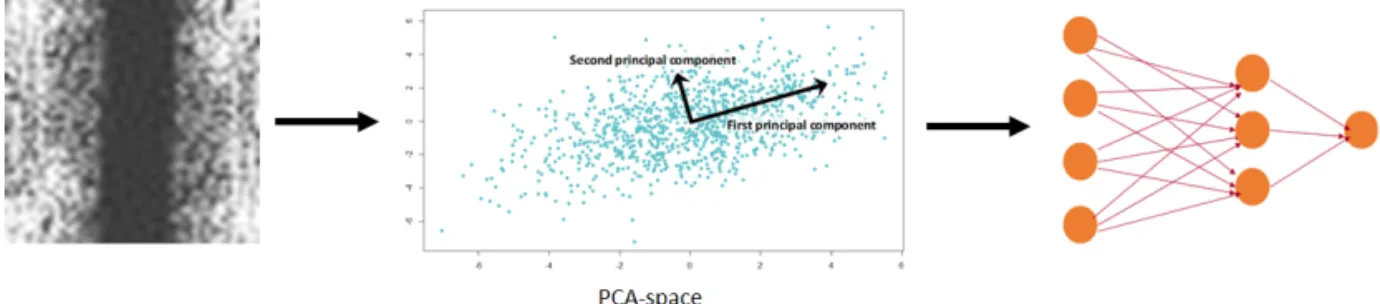
The outputs of the classifier will represent the final diagnosis of the system. A schematic representa- tion of the proposed diagnosis system is shown in Fig. 1.

The final results demonstrate that the method presented in this paper manages to capture the in- ner characteristics of the data by discovering the existing differences between them. We demon- strate also how the conventional statistical features dramatically fail to capture those differences.

Although the time-frequency based features pre- sented in [9] also manage to seize the character- istics of the data, we demonstrate that our method still outperforms them in case of the sounds pro- duced by the drills.

In the following section, we will present in de- tails the problem treated by this publication and al- so discuss the proposed method. In section 3, we

present the detailed results obtained during the ex- periments and we also conduct a detailed com- parative study between our method and other fea- ture extraction methods.

2. PROPOSED MFD METHOD

The problem considered in this work is the auto- matic detection of the damaged drills during their working time and using the sounds they produce.

The assessment system we want to build must be able to recognize automatically whether the sound was produced by a healthy or a faulty drill. All the purpose of this work is to present a method able to find the differences between a sound from a healthy drill and a sound from a faulty drill, in an automatic way. The feature extraction method that we present here is mainly based on the idea of ex- tracting the magnitude spectrum of the sounds and representing them as images. Then, those images will be furtherly processed and used as the features of our system. Fig. 1 summarizes the principal steps used in this method.

2.1 Extraction of the magnitude spectrum The collected data sounds are one-dimensional

discrete vectors containingN sampling points and represented by x(n). The discrete Fourier trans- formX(k) of the discrete signals x(n) can be com- puted by using the following equation

 



  

  

 ^{ } (1)

where the values of k represent the frequency components of the original signalx(n). Thus, X(k) is the representation of the time seriesx(n) in the frequency domain. The second part of this equation comprises a complex number that can be decom- posed in a sum of sines and cosines, as shown in the following equation

 _{  }^{  }^{}_^cos













^^^^{ }^{  }^ (3) The magnitude spectrum is the function de- scribing the magnitude of every single frequency.

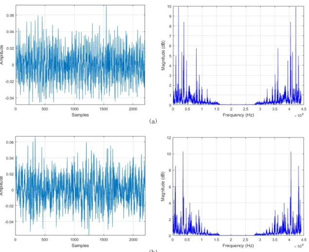
In Fig. 2 we show some sample data (sounds) from our database and their corresponding magnitude Fig. 1. Representation of the proposed method.

spectrum. In Fig. 2 (a) we have one of the normal data, which are the data collected via the healthy drill. In the left we show the data and on its right we have its magnitude spectrum. In Fig. 2 (b) we see one of the abnormal data, which are the data collected using the damaged drill. In the left we have the sound data and on its right, we have cor- responding magnitude spectrum. We can notice how the useful information is located mainly in the low frequency band for both data.

2.2 Image conversion

The next step after computing the magnitude spectrum of the data is to convert them into images. As we can clearly see in Fig. 2, the sounds are one-dimensional data. Using equation (3) to compute the magnitude spectrum of each fre-

quency component also gives a one-dimensional vector. Images being two-dimensional vectors, the next step of our method is to map the one-dimen- sional magnitude spectrum vectors to some two-dimensional vectors. The vectors containing the magnitude values are segmented in many dif- ferent parts. These segmented parts are then used as columns in order to create the two-dimensional matrices that we want. According to the images shown in Fig. 2, most of the significant values are located at the two opposite extremities of the mag- nitude vectors. These values will also be located among the columns positioned at the ends of the matrices. The conversion process just consists of dividing the vectors in different parts and position- ing those parts as columns in order to create a two-dimensional matrix. Other remaining details

(a)

(b)

Fig. 2. (a) Normal sound data and its corresponding magnitude spectrum, (b) abnormal sound data and its corre- sponding magnitude spectrum.

about the conversion will be discussed in the next section.

The magnitude are small values mostly located between 0 and 20, as we can see in the examples shown in Fig. 2. The next step of our method is to normalize the created 2D matrices in such a way that they can be represented as 8-bit grayscale images. We have linearly normalized the matrices using the next following equation

_ _{ }

 

  

  (4) where the values I are the actual values of the magnitude spectrum that we have in the 2D ma- trices, and the values Inor represent the values of the normalized matrices. Max and Min represent respectively the maximum and minimum values of the extracted magnitude spectrum.nMax and nMin are respectively the new maximum and new mini- mum that we want for the image conversion. As we aspire to obtain 8-bit grayscale images, the new maximum and minimum are set to 255 and 0, respectively, in equation (4). After applying the equation to every single matrix containing the magnitude spectrum, we obtain 8-bit grayscale images. Because most of the values are really small and zero in the vectors containing the magnitude spectrum, the created images are composed of mostly black pixels. The high values located at the extremities of the vectors will represent the white pixels in the created images and are also located at the two ends of the images.

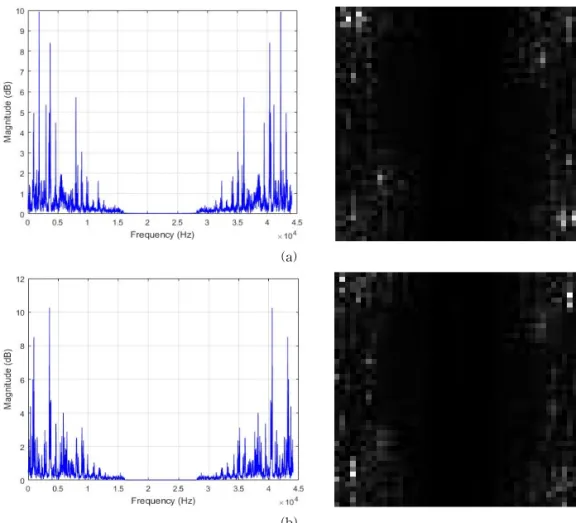
In Fig. 3, we show the created images using the data samples shown in Fig. 2. In Fig. 3 (a), we have in the left the magnitude spectrum of the normal data shown in Fig. 2 (a) and the corresponding ob- tained image after using equation (4), shown in the right. In Fig. 3 (b), we have in the left the magni- tude spectrum of the abnormal data shown in Fig.

2 (b) and the corresponding obtained image shown in the right. We can notice that most of the pixels of the images are black, or in the low intensity band, as we see in their histograms shown in Fig.

4. The most important factor to understand and to keep in mind is that the useful information that we want in order to understand the data are all located in the low frequency band of the magnitude spec- trum, thus, in the white pixels of the created images. The next step is to find a way to spread all over the images the information about the health.

2.3 Contrast adjustment using histogram equal- ization

As explained before, the characteristics of the data mostly lay on the extremities of the vectors containing the magnitude spectrum, which are the low frequency values. The low frequency values contain all the details and aspects of the machines’

health condition, which actually represent all the information that we need in order to recognize the condition automatically. In order to reinforce those characteristics, we propose to spread them all over the images. Histogram equalization [11] has the ability to correct the contrast of the images by uni- formly disseminating the gray intensity for all the pixels. Applying histogram equalization on our created images will have as effect of spreading the information that is now located only at the ex- tremities (the low frequency band) over all the images. Consequently, this effect will reinforce the health information by revealing the hidden charac- teristics of the data.

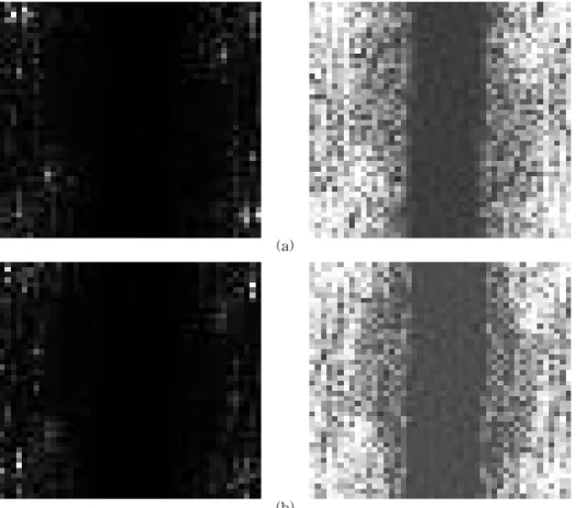
In Fig. 5 we show the results obtained by apply- ing histogram equalization on our created images.

The most important factor to mention about the obtained histogram equalized images is that we can feel, even by a quick visual inspection, the differ- ences between the normal and abnormal data.

When we look at the time series shown in Fig. 2, we cannot really remark the differences between them, and even when we look at the images created using the linear normalization, the differences are unclear and difficult to seize, the two kinds of data being largely similar. But the fact of spreading the

health information located at the low frequency band and at the extremities of the images really transform the images in such a way that all the information about the health’s state of the sound

is scattered in the images. Fig. 6 shows the histo- grams of the histogram equalized images, and we can see how all the pixel intensity are represented.

The contrast adjustment process will force the (a)

(b)

Fig. 3. The magnitude spectrum of the data and their corresponding normalized image: (a) a normal data, and (b) an abnormal data.

(a) (b)

Fig. 4. Histogram of the images in Fig. 3, (a) the normal data and (b) the abnormal data.

image data from a given kind of drill to be really similar between them, and thus, different to the images obtained using the other drill. Therefore, the histogram equalized images shown in Fig. 5 will be adopted as the features for our machine fault detection analysis. Those images will be re-

duced with PCA and given to a neural network classifier for the final output of the assessment system.

2.4 Dimensionality reduction

PCA [12] is a statistical procedure that uses an

(a) (b)

Fig. 6. Histogram of the contrast enhanced feature images: (a) the normal data and (b) the abnormal data.

(a)

(b)

Fig. 5. Feature images with their corresponding histogram equalized output: (a) the normal data and (b) the abnormal data.

orthogonal transformation in order to convert a set of correlated data into a set of values that are line- arly uncorrelated. Those values are called principal components. The number of the obtained principal components is less than or equal to the dimension of the original data. PCA is defined in such a way that the first principal component has the largest possible variance, which makes it to be sensitive to the variability of the dataset. Each succeeding component in turn must also have the highest var- iance possible under the constraint that it must be orthogonal to the preceding components. The ob- tained vectors from the principal components will be used as a new basis, called the PCA-space, on which we will project the original data in order to obtain their new representation. That is the part of dimensionality reduction capability of the PCA.

In this paper, we will compute the PCA-basis using the feature images shown in Fig. 5 (the his- togram equalized images) as the original data. After projecting the feature images into the PCA- space, some projections will be selected in order to be given to a nonlinear classifier, as shown in Fig. 7.

2.5 Classification with artificial neural network Artificial neural networks (ANNs) [13] consist of interconnected group of artificial neurons in which the information flows from the starting neu- rons to the ones located at the far end of the network. The information flows using some non- linear functions whose purpose is to discover some nonlinearities contained inside the data in order to

use them for the comprehension of those data.

ANNs are adaptive systems that learn to change their structure based on the received information and acquire the ability to generalize the learned comprehension after the learning process. The net- works learn by back-propagating the errors [14]

between the actual outputs and the desired ones.

In this paper, the selected projections of the feature images will be given to a neural network based classifier whose output will represent the final di- agnosis of the MFD system.

3. RESULTS AND DISCUSSION

We have collected data sounds from healthy and damaged drills using a microphone. Sound being a nonstationary signal, we have segmented the re- corded data into many different parts in order to construct our dataset for the pattern recognition step. The used sampling frequency and signal length were 44100Hz and 0.05 s, respectively. We have created a dataset of 2183 data sounds, 1120 from the healthy drill and 1063 data from the dam- aged drill. We have first started by computing the magnitude spectrum of each recorded sound. Using the sampling frequency and the signal length men- tioned above, each sound is a vector containing 2205 points, as we can see in Fig. 2. From equation (1), we see that the DFT vectors also will contain 2205 elements. The DFT are evaluated for the fre- quency from 0 Hz to 22050 Hz due to the Nyquist theorem, and each DFT value from 22050 Hz to 44100 Hz is a replication of the previously com-

Fig. 7. Pattern recognition part of the MFD system: dimensionality reduction using PCA and neural nonlinear classifier for the final step.

puted values. Using equation (3) to estimate the magnitude of each frequency component gives the vectors shown in Fig. 2.

To estimate the two-dimensional vectors, we can first notice that 2205 = 49×45 and, following this fact, we have segmented each magnitude spectrum vector into 45 parts of length 49. We have 45 49-dimensional vectors that we will use as the columns of the 2D matrices that we want to create.

Which gives two-dimensional matrices of size

49×45. After the linear normalization process, we obtain 49×45 8-bit grayscale images. Having 2183 data sounds in origin, the feature images that we will be handling form the matrix of size 49×45×2183.

Then, finally, histogram equalization will be ap- plied over the created feature images in order to adjust their contrast and spread the health patterns all over the images. Some of the obtained images are shown again in Fig. 8.

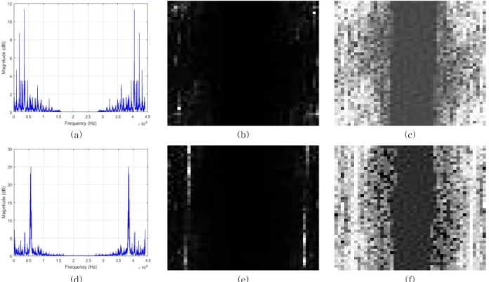
We can see in Fig. 8 how the histogram equal-

(a) (b) (c)

(d) (e) (f)

Fig. 8. Some feature images obtained during the experiments: in the first line (a, b, and c) we have a normal data and in the second line (d, e, and f) we have an abnormal data.

(a) (b)

Fig. 9. Image difference between the normal and abnormal feature images shown in Fig. 8: (a) using the images created only with the magnitude spectrum, and (b) using the histogram equalized images.

ization increases the differences between the two kinds of data. In Fig. 9, we show the image differ- ence between the normal and abnormal feature im- ages shown in Fig. 8. In Fig. 9 (a), the difference was obtained using the images created with the magnitude spectrum, and in Fig. 9 (b), the differ- ence was obtained using the histogram equalized images, our feature images. We can see that the images created using only the magnitude spectrum suffer a lack of information, while the difference is maximized after adjusting the contrast.

As we have explained in the beginning of this discussion, the sounds data are corrupted by some disturbances from the environment sites that make

them to be non-distinguishable. We can see it in Fig. 10, where we show the projections of the data using their raw time series. We can remark how the data are very much similar, and how they are all clustered together. The statistical features do not help, as shown in Fig. 11.

Once we use our created feature images, we can remark how the projections of the data show the differences between the normal and abnormal sounds. In Fig. 13, we show the data using the fea- ture images created with only the magnitude spectrum. The feature images really capture the differences between the 2 data, as we can notice.

Even though the projections are good, because they really show the differences between the data, we can obtain much clearer projections by using the histogram equalized images. In Fig. 14, we show the projections using our final feature images, the contrast enhanced images and we can see how the data are properly separated, creating two distinct clusters.

The projections shown in Fig. 14 were used as the inputs of the neural network based classifier.

For every single data, we have selected the 3 fea- tures represented by the 3 axis in the projections shown in Fig. 14: the first, second and third princi- pal components (PC). The network has 3 layers.

The input layer comprises 3 neurons according to

Fig. 12. Normal and abnormal data using the DWT co- efficients, as proposed in [9].

Fig. 10. Normal and abnormal data sounds using their time series.

Fig. 11. Normal and abnormal data sounds using their statistical features as computed in [7].

the 3 features, the hidden layer has 5 neurons, and we have 2 neurons in the final layer, according to the two instances that we have, the normal and abnormal data. Each neuron uses the sigmoid function defined by   tanh as the learn-

ing function. We recall that we have used 2183 da- ta, 70% of them were used for the training and the remaining 30% were used for testing the trained network. The obtained results are shown in Table 1.

By analyzing Table 1, we see that the total accu- racy of the classifier reaches 99.5 %. It is not sur- prising because the data given to the classifier are the data shown in Fig. 14. These data are really different, forming completely 2 different clusters.

Even a simple linear classifier can well separate them. We have adopted the nonlinear classifier in order of maximizing the separation, reaching 99.5

%. In details, considering the normal data as pos- itive and the abnormal as negative data, we can see the true positive rate obtained by the classifier.

Which means that the classifier perfectly recog- nizes the normal data between them, and only a few of them were misclassified. The false positive rate also is really small (0.003), which means the classifier recognizes the quasi totality of the ab- normal data.

The comparative study contains the method presented in [7], where the statistical features were computed using the time series of the data. We can see that the false positive rate is big, which means that the classifier has trouble to recognize the ab- normal data, many of them being misclassified.

The projections of the data using this method can be seen in Fig. 11. The discrete wavelet transform (DWT) coefficients as used in [9] and the con- tinuous wavelet transform (CWT) coefficients as proposed in [10] represent the time-frequency do- main based analysis. We recall that our method is mainly based on the frequency domain by extract- Table 1. Results summary

References [7] [9] [10] Present work

Feature Extraction

Method Time series +

statistical features DWT coefficients

+ PCA CWT components +

statistical features Feature images Classifier Neural network Neural network Neural network Neural network

True positive rate 0.924 0.975 0.873 0.993

False positive rate 0.198 0.061 0.356 0.003

Total accuracy 86.1 % 95.7 % 75.8 % 99.5 %

Fig. 13. Normal and abnormal data using the feature im- ages created with only the magnitude spectrum.

Fig. 14. Normal and abnormal data using the contrast enhanced feature images.

ing the magnitude spectrum of the sounds before converting them into images. Even though the DWT coefficients reach a total of 95.7 %, as we could have expected by analyzing the projections shown in Fig. 12, they are still outperformed by the proposed method in this paper. On the other hand, the CWT coefficients have failed to well rec- ognize the abnormal data, as we can see in Table 1, with the false positive rate of the classification using this method increasing to 0.356.

4. CONCLUSION

The method proposed in this study proves that it can reach outstanding performance in pattern recognition based fault diagnosis of drills using sounds. We have presented a novel feature ex- traction method that extracts the magnitude spec- trum of the sounds before converting them into images. We saw how difficult can be the analysis in the time domain because the recorded sounds are disturbed by the noises. Our proposed feature extraction manages to expose the existing differ- ences between the normal and abnormal data. After converting the magnitude spectrum into images, we have applied histogram equalization in order to correct the contrast of the created images and also spread all over them the information previously concentrated in the low frequency band of the sounds. The created feature images are projected to the PCA-space and the first 3 projections are selected in order to be given to the nonlinear classifier.

Compared to the time domain and the time-fre- quency domain provided by the DWT and CWT coefficients, our feature images coefficients ac- complishes outstanding performance by capturing the main characteristics of the data. The method presented here can be used in any other fault diag- nosis system. If it can separate normal and abnor- mal sounds of the drills, it can be also used for vibrations and other acoustic emission data.

REFERENCE

[ 1 ] M.M. Polycarpou and A.T. Vemuri, “Learning Methodology for Failure Detection and Acc- ommodation,”IEEE Control Systems, Vol. 15, No. 3, pp. 16-24, 1995.

[ 2 ] N.R. Sakthivel, V. Sugumaran, and B.B. Nair,

“Application of Support Vector Machine (SVM) and Proximal Support Vector Machine (PSVM) for Fault Classification of Mono Block Centri- fugal Pump,” International J ournal of Data Analysis Techniques and Strategies, Vol. 2, No. 1, pp. 38-61, 2010.

[ 3 ] Y. Xu and H. Wang, “A New Feature Selec- tion Method Based on Support Vector Ma- chines for Text Categorization,”International J ournal of Data Analysis Techniques and Strategies, Vol. 3, No. 1, pp. 1-20, 2011.

[ 4 ] N.R. Sakthivel, B.B. Nair, V. Sugumaran, and R.S. Rai, “Application of Standalone System and Hybrid System for Fault Diagnosis of Centrifugal Pump Using Time Domain Signals and Statistical Features,”International Journal of Data Mining Modeling and Management, Vol. 4, No. 1, pp. 74-104, 2012.

[ 5 ] N. Tandon and B.C. Nakra, “Vibration and Acoustic Monitoring Techniques for the De- tection of Defects in Rolling Element Bearings -A Review,”The Shock and Vibration Digest, Vol. 24, No. 3, pp. 3-11, 1992.

[ 6 ] C. Vununu, J.H. Park, S.H. Lee, and K.R.

Kwon, “Sound Based Machine Fault Diagno- sis System Using Pattern Recognition Tech- niques,”Journal of Korea Multimedia Society, Vol. 20, No. 2, pp. 134-143, 2017.

[ 7 ] P.K. Kankar, S.C. Sharma, and S.P. Harsha,

“Fault Diagnosis of Ball Bearings Using Machine Learning Methods,”Expert Systems with Applications, Vol. 38, No. 3, pp.

1876-1886, 2011.

[ 8 ] B. Samanta, K.R. Al-Balushi, and S.A. Al- Araimi, “Artificial Neural Networks and Gen- etic Algorithm for Bearing Fault Detection,”

Soft Computing, Vol. 10, No. 3, pp. 264-271, 2006.

[ 9 ] K.M. Lee, C. Vununu, K.S. Moon, S.H. Lee, and K.R. Kwon, “Automatic Machine Fault Diagnosis System Using Discrete Wavelet Transform and Machine Learning,”Journal of Korea Multimedia Society, Vol. 20, No. 8, pp.

1299-1311, 2017.

[10] P.K. Kankar, S.C. Sharma, and S.P. Harsha,

“Fault Diagnosis of Ball Bearings Using Con- tinuous Wavelet Transform,” Applied Soft Computing, Vol. 11, No. 2, pp. 2300-2312, 2011.

[11] J.C. Russ,The Image Processing Handbook:

Forth Edition, CRC Press, Florida, Boca Raton, 2002.

[12] K. Pearson, “On Lines and Planes of Closest Fit to Systems of Points in Space,” Philo- sophical Magazine Series 6, Vol. 2, No. 11, pp. 559-572, 1901.

[13] M.J. Zurada,Introduction to Artificial Neural Systems, Jaico Publishing House, Delhi, 1999.

[14] D.E. Rumelhart, G.E. Hinton, and R.J. Wil- liams, “Learning Representations by Back- propagating Errors,” Nature, Vol. 323, No.

6088, pp. 533-536, 1986.

Caleb Vununu

He received his B.S. degree in Computer Science in Youngsan University, Republic of Korea in 2015. Since September 2015, he’s a Master degree student in the department of IT Convergence and Application Engineering in Pukyong National University. His research interests include Signal Processing and Machine Learning.

Oh-Heum Kwo

He received the BS degree in computer engineering from Seoul National University in 1988, and the MS and PhD degrees in computer science from the Ko- rea Advanced Institute of Sci- ence and Technology in 1991 and 1996, respectively. He is currently a professor in the Dept. of IT Convergence and Application Engin- eering at the Pukyong National University, Pusan, Republic of Korea. His research interests include de- sign and analysis of algorithms and distributed com- putting.

Kwang-Seok Moon He received the B.S., or Studies M.S., and Ph.D. degrees in Elec- tronics Engineering in Kyung- pook National University, Korea in 1979, 1981, and 1989 respec- tively. He is currently a pro- fessor in department of Electro- nic engineering at Pukyong National University. His research interests include digital image processing, video watermarking, and multimedia communication.

Suk-Hwan Lee

He received a B.S., a M.S., and a Ph. D. degrees in Electrical Engineering from Kyungpook National University, Korea in 1999, 2001, and 2004 respec- tively. He is currently an asso- ciate professor in Department of Information Security at Tongmyong University. His research interests include multimedia security, digital image processing, and computer graphics.

Ki-Ryong Kwon

He received the B.S., M.S., and Ph.D. degrees in electronics en- gineering from Kyungpook Na- tional University in 1986, 1990, and 1994 respectively. He work- ed at Hyundai Motor Company from 1986-1988 and at Pusan University of Foreign Language from 1996-2006. He is currently a professor in Department of IT Convert- gence and Application Engineering at the Pukyong National University. He has researched University of Minnesota in USA in 2000-2002 with Post-Doc. and Colorado State University on 2011-2012 with visiting professor. He was the President of Korea Multimedia Society in 2015-2016. His research interests are in the area of digital image processing, multimedia security and watermarking, bioinformatics, weather radar in- formation processing, and machine learning.