Predicting Future Terrestrial Vegetation Productivity Using PLS Regression

Predicting Future Terrestrial Vegetation Productivity Using PLS Regression*

Chul-Hyun CHOI

·Kyung-Hun PARK

·Sung-Gwan JUNG

PLS 회귀분석을 이용한 미래 육상 식생의 생산성 예측*

최철현

·박경훈

·정성관

*

ABSTRACT

Since the phases and patterns of the climate adaptability of vegetation can greatly differ from region to region, an intensive pixel scale approach is required. In this study, Partial Least Squares (PLS) regression on satellite image-based vegetation index is conducted for to assess the effect of climate factors on vegetation productivity and to predict future productivity of forests vegetation in South Korea.

The results indicate that the mean temperature of wettest quarter (Bio8), mean temperature of driest quarter (Bio9), and precipitation of driest month (Bio14) showed higher influence on vegetation productivity. The predicted 2050 EVI in future climate change scenario have declined on average, especially in high elevation zone. The results of this study can be used in productivity monitoring of climate-sensitive vegetation and estimation of changes in forest carbon storage under climate change.

KEYWORDS : Climate Change, MODIS EVI, Bioclimatic Variables, PLS Regression

요 약

식생의 기후 적응력은 지역에 따른 상황 및 공간적 패턴이 다르게 나타나기 때문에 픽셀 스케일 의 접근이 필요하다. 본 연구에서는 위성영상 기반 식생지수에 대해 PLS 회귀분석을 적용하여 식 생의 생산성에 영향을 미치는 기후요인을 평가하고 남한지역의 미래 산림 생산성을 예측하였다.

그 결과, 최고강수분기의 평균기온(Bio8), 최저강수분기의 평균기온(Bio9), 최저강수월의 강수량

2016년 12월 16일 접수 Received on December 16, 2016 / 2017년 2월 1일 수정 Revised on February 1, 2017 / 2017년 2월 6일 심사완료 Accepted on February 6, 2016

* This work was supported by the National Research Foundation of Korea(NRF) grant funded by the Korea government (MSIP) (No. NRF-2016R1A2B4015460).

1 국립생태원 생태보전연구실 Division of Ecological Conservation, National Institute of Ecology 2 창원대학교 환경공학과 Department of Environmental Engineering, Changwon National University 3 경북대학교 조경학과 Department of Landscape Architecture, Kyungpook National University

※ Corresponding Author E-mail : [email protected]

(Bio14) 변수가 식생의 생산성에 높은 영향을 미치는 것으로 분석되었다. 미래 기후시나리오 자료 를 이용하여 예측된 2050년의 식생 생산성은 전체적으로 감소하는 것으로 나타났으며, 특히 고지 대에서 크게 감소하는 것으로 분석되었다. 이러한 결과는 기후에 민감한 지역의 식생에 대한 생산 성 모니터링과 미래 기후변화로 인한 산림 탄소 저장량의 변화를 평가하는데 있어 유용하게 활용 될 수 있을 것으로 판단된다.

주요어 : 기후변화, MODIS EVI, 생물기후변수, PLS 회귀분석

INTRODUCTION

Plants produce energy through photosy- nthesis and fix organic carbon, and can be used as the most fundamental energy for growth and maintenance of various other organisms(Bryant et al., 1983). Also, pree- xisting vegetation interacts with the abiotic environment, greatly affecting the resource and habitats of other populations inside the ecosystem (Turner et al., 2001).

Climate is the major factors affecting the performance of terrestrial ecosystems.

According to the 4th IPCC report, the mean temperature of the Earth for the past 100 years(1906-2005) increased by approximately 0.74℃(Barker et al., 2007), and the 5th IPCC report states that, if this trend continues for the next 100 years, the mean temperature at the end of the 21st century will have increased by 3.7℃

compared to the years of 1986-2005, with serious damages to ecosystem(Melillo et al., 1993).

When the climate changes, the produc- tivity of vegetation which is sensitive to the climate conditions, is also altered.

Therefore, monitoring vegetation conditions and productivity in ecosystem under climate change is very important. Many studies were conducted to analyze climate sensitivity of vegetation by investigating

the relationship between growth and climate (Thammincha, 1981; Henttonen, 1984;

Kalela-Brundin, 1999; Ha et al., 2007;

Choi et al., 2016).

In the past, the productivity of vegetation was inferred from the time series growth data of trees, which were analyzed with dendrochronology. However, dendrochron- ological investigation is a destructive method that requires the growth ring of wood specimen with mechanical damage to trees.

Also field-based investigation requires much time and effort, thus long-term research against a wide range of forests areas is almost impossible.

Alternatively, the relationship between the vegetation index derived from satellite image and vegetation productivity was introduced in recent study with reports that the vegetation index and productivity are highly related(D'arrigo et al., 2000;

Wang et al., 2004; He and Shao, 2006;

Lopatin et al., 2006; Choi and Jung, 2014).

Therefore, it would be efficient if remote sensing techniques were used for the study of vegetation productivity over large areas.

The Global Inventory Modeling and Mapping

Studies (GIMMS) NDVI from the Advanced

Very High Resolution Radiometer (AVHRR)

is useful for the studies of temporal

changes in vegetation productivity and this

data have been collected continuously

since 1981. However, since its spatial

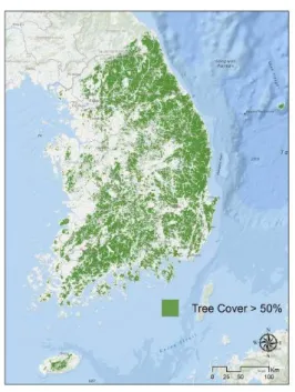
FIGURE 1. Map of the study site.

Forest cover extracted from MOD44B (tree cover > 50%)

resolution is low(1㎞), it is not suitable for the local scale studies. Meanwhile, the veg- etation index data derived from Moderate Resolution Imaging Spectrora- diometer(MODIS) have the spatial reso- lution of approximately 250m. Therefore, MODIS products made it possible to derive differences of vegetation productivity in a small watershed(2㎢) that have relatively homogeneous environmental conditions in forests(Chang, 2012). Also, the MODIS data archive contains the data for more than 10 years, which is advantageous for time series analysis.

In this study, major climate factors influencing vegetation productivity are determined using MODIS vegetation index and climate data. Furthermore, we predi- cted future productivity in order to identify areas vulnerable to climate change.

DATA AND METHODS

1. Study Area

The spatial scope of the study is South Korea, located in middle-latitudes with a temperate climate zone and four distinctive seasons. South Korea has a small land area, but its complex geography, seasonal changes and many different types of biomes make the climatic influence quite different from region to region. About 63%

of the land area is covered with forests that have various biome types including temperate evergreen forests, temperate deciduous forests and subalpine needle- leaved forests, etc. Therefore, the relati- onship between vegetation productivity and climate needs to be further studied. Only forest areas were extracted for the analysis

using MODIS Terra MOD44B tree cover data with values above 50%(Figure 1).

2. MODIS EVI time series

Estimating forest productivity through field surveys has many limitations when considering budgets and manpower. The remote sensing-based ecosystem monitoring method can be an excellent alternative.

MODIS is the sensor aboard the National Aeronautical and Space Administration’ s (NASA) Terra and Aqua Earth Obser- vation System(EOS) satellites, which provide land, oceans and atmosphere monitoring data, and have been commonly used in recent ecosystem studies. The MODIS vegetation index data is useful for evaluating the photosynthesis activity through chloro- phyll contained within the leaves of plants.

The Normalized Difference Vegetation

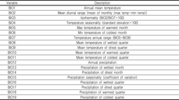
Variable Description

BIO1 Annual mean temperature

BIO2 Mean diurnal range (mean of monthly (max temp-min temp))

BIO3 Isothermality (BIO2/BIO7×100)

BIO4 Temperature seasonality (standard deviation×100)

BIO5 Max temperature of warmest month

BIO6 Min temperature of coldest month

BIO7 Temperature annual range (BIO5-BIO6)

BIO8 Mean temperature of wettest quarter

BIO9 Mean temperature of driest quarter

BIO10 Mean temperature of warmest quarter

BIO11 Mean temperature of coldest quarter

BIO12 Annual precipitation

BIO13 Precipitation of wettest month

BIO14 Precipitation of driest month

BIO15 Precipitation seasonality (coefficient of variation)

BIO16 Precipitation of wettest quarter

BIO17 Precipitation of driest quarter

BIO18 Precipitation of warmest quarter

BIO19 Precipitation of coldest quarter

TABLE 1. Description of bioclimatic variables.

Index (NDVI) was developed to capture the characteristic in which chlorophyll strongly absorbs the visible light(0.45-0.67µm), and reflects the near-infrared light(0.74-1.3µm) (Rouse et al., 1973). MODIS includes the NDVI along with the Enhanced Vegetation Index(EVI). The EVI uses the blue band to remove residual atmosphere contam- ination and maintains sensitivity over dense vegetation conditions.

In this study, the MODIS EVI(MOD13Q1) data were used to evaluate the vegetation productivity. MOD13Q1 data are provided every 16 days at 250m spatial resolution.

The mean EVI values were calculated from 2000 to 2014 for all pixels.

3. Bioclimatic variables

To determine the relationship between climate and vegetation productivity, climate data which is closely related to the growth of the vegetation is required. Bioclimatic

variables were derived from climate data to better represent the types of seasonal trends pertinent to the physiological constraints of different species(O’Donnell and Ignizio, 2012). There are 19 biocli- matic variables to considers the annual trends, seasonality, extreme or limiting environmental factors(Table 1). In order to create bioclimatic variables, historical records from weather stations are needed.

There are 571 Automated Weather Station (AWS) operated by the Korea Meteoro- logical Administration in South Korea. By using all of the AWS records, nearly 12km-resolution climate surfaces derived across the study site. However, climate data at a fine spatial resolution are necessary to capture the environmental variability, so an appropriate spatial interpolation is required.

Generally, the spatial interpolation of

temperature is invariably influenced by

elevation(DeGaetano and Belcher, 2007).

To consider variations of temperature by elevation and local topographic differences, the Geographically Weighted Regression (GWR) method was used in this study.

GWR sets the elevation derived from the Digital Elevation Model (DEM) as the independent variable, and the monthly maximum temperature and monthly mini- mum temperature in the AWS records as the dependent variable. Cross-Validation (CV) technique was used for bandwidth optimi- zation (Fotheringham et al., 2003; Bivand et al., 2015). The DEM data was obtained from the 30m-resolution Advanced Space- borne Thermal Emission and Reflection Radiometer(ASTER) Global Digital Elevation Model Version 2(GDEM V2) provided by the NASA. The analysis was conducted using the 'spgwr' package of R(Team, 2013;

Bivand et al., 2015). The precipitation data were interpolated using Inverse Distance Weighting(Yang et al., 2015). As a result of verifying the accuracy with Root Mean Square Error (RMSE) for the interpolation data, the mean RMSE of the precipitation, maximum temperature and minimum tem- perature are 28.76, 0.74, 1.02, respectively.

Both temperature and precipitation grid data were all assembled as raster layer with spatial resolution of 250m. The bioclimatic variables were derived using the R 'dismo' package(Hijmans et al., 2016). The input data are the monthly precipitation, maximum temperature and minimum temperature of the grid meteo- rological data processed through spatial interpolation using AWS records.

4. PLS regression

To estimate the magnitude of the influence

of the bioclimatic variables in affecting the vegetation productivity, Partial Least Squares (PLS) regression analysis was conducted, instead of traditional regression analysis. PLS regression analysis is especially suitable for numerous variables with few observed values(Cramer et al., 1988). Since the PLS regression analysis includes latent factors, which are inde- pendent from each other when cons- tructing a model, it is free from the issue of multicollinearity problems. Also, the model’s parsimony can be increased, because the latent factors are extracted from the predictors a set of orthogonal factors which have the best predictive power(Wold et al., 2001). The optimized number of latent factors can be determined by calculating the Predictive Residual Sum of Squares(PRESS) through 5-fold Cross -Validation(CV). The model with the number of latent factors giving lowest PRESS is then used. To avoid overfitting, latent factors was set from 1 to 10 (Luedeling and Gassner 2012; Yu et al., 2012).

Differential influence of bioclimatic variables on vegetation productivity can be determined by Variable Importance in the Projection(VIP) scores that appear in the output for PLS regression analysis.

Generally, when the VIP score is over 1, it can be defined as a statistically significant variable and considered as an important variable for estimating the relationship (Wold et al., 2001).

When a regression coefficients was

derived by the PLS regression analysis,

future EVI can be estimated using future

bioclimatic variables. In this study, future

FIGURE 2. The ratio of the areas with VIP scores above 1 in all forests of South Korea.

All forest areas were classified into areas with VIP>1 and VIP<1 for each variable, and the ratio of the areas with VIP>1 were calculated (see Figure 3).

bioclimatic variables in 2050 of the RCP 8.5 scenario(HadGEM2-AO) provided by Worldclim-Global Climate Data(www.worldclim.

org) were used. The PLS regression analysis was conducted for each pixel in order to consider differences of the climatic sensit- ivity for the each biome types and regions.

The PLS regression analysis for all pixels performed using the‘mixOmics’package (Le Cao et al., 2015) and the‘raster’package (Hijmans et al., 2015).

RESULTS AND DISCUSSION

1. Importance of the Climatic Factors Affecting Productivity of the Vegetation As a result of verifying the accuracy of the PLS model, the mean absolute error, root mean squared error and correlation coefficient were 0.008, 0.011, 0.966 res- pectively. The VIP scores, which reflects

the importance of bioclimatic variables on EVI, are classified into threshold of 1 for all pixels. Then, the ratios of the areas with VIP scores above 1 were calculated for each bioclimatic variables(Figure 2).

Bio8, Bio9, and Bio14 variables which refer to the mean temperature of wettest quarter, mean temperature of driest quarter, and precipitation of driest month, respe- ctively, showed that the ratio is over 50%.

In predicting a species distribution or productivity change, average annual tem- perature or annual precipitation have mainly been used(Austin et al. 1990; Miao et al.

2015). However, based on the above

findings, the temperature and precipitation

of specific monthly or quarterly periods must

be considered as more important than the

averaged annual values. Meanwhile, Bio4,

Bio11, and Bio12 variables which refer to

the temperature seasonality, mean tem-

perature of coldest quarter, and annual

(a) Bio8 (b) Bio9

(c) Bio14 (d) Bio4

FIGURE 3. Maps of reclassified VIP scores for the bioclimatic variables

FIGURE 4. Mean VIP scores of bioclimatic variables for the annual precipitation.

precipitation, respectively, showed that ratio is below 30%.

Since the distribution map of the signi- ficance VIP scores for all 19 bioclimatic variables, major influential limiting climate factors in relation to the vegetation prod- uctivity for certain areas can be determi- ned(Figure 3a-c, other variables not shown on the maps). In the case of Bio4 variable, ratio is 22% that reflecting its lower impo- rtance relative to other factors. However, the importance of the Bio4 variable was high in certain areas (red-colored regions in Figure 3d), and we can interpret that the Bio4 variable will have a large effect on productivity in these regions(Figure 3d).

The mean VIP scores of the bioclimatic variables for the elevation categories are shown in Figure 4. High elevation areas have higher VIP scores than low elevation areas in Bio10 variable, which refers to the mean temperature of warmest quarter.

High elevation zone are mainly populated with plants that are adapted to low temperature, so the influence of the high temperature in hot summer season can be

higher than lower elevation areas. The comparatively lower thermotolerance of the high elevation species have been reported in previous studies(Smillie et al., 1983;

Valcu et al., 2008).

The mean VIP scores of the bioclimatic variables for the annual precipitation, Bio5 and Bio8 variables, which refer to the max temperature of warmest month, and mean temperature of wettest quarter, respectively, were especially higher in the regions with relatively low precipitation zone(<1,200

㎜)(Figure 5). To interpret relationship between climate factors and productivity of vegetation, interaction between temperature and water stress must be considered. In particular, the rise in temperature during droughts, plants stomatal closure takes place to avoid loss of water due to excessive evaporation. Prolonged stomatal closure aggravates the carbon-starvation of plants(McDowell et al., 2008). Therefore, temperature during low precipitation periods, can be a very important limiting factor on vegetation productivity.

When we compared the VIP scores of

FIGURE 6. Mean VIP scores of bioclimatic variables for the each forest types.

FIGURE 5. Mean VIP scores of bioclimatic variables for the elevation categories.

the bioclimatic variables for the each forest types, the mean VIP scores of the Bio5, Bio10, Bio15 variables, which refer to the max temperature of warmest month, mean temperature of warmest quarter, and precipitation seasonality, respectively, were much higher in evergreen broad-leaf forests than other forest types(Figure 6).

Similarly, Bowman et al.(2014) reported that high temperature in warmest month will reduce tree growth in evergreen

broadleaf forests through their effect on evaporation and water availability.

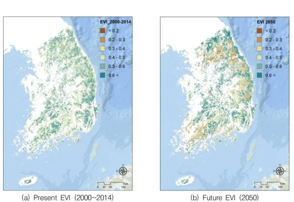
2. Estimating Future EVI Under Climate Change

The mean EVI between 2000~2014

(present) and future EVI(2050) estimated

from PLS regression model is shown in

Figure 7a and 7b. The present EVI value

is 0.50, and the future EVI is 0.48 on

(a) Present EVI (2000~2014) (b) Future EVI (2050)

FIGURE 7. Spatial distribution of EVI in (a) present, (b) future and (c) future-present difference

(c) Future-present EVI FIGURE 7. Continued

average, which indicates a decrease in the future. Figure 7c shows the results obtained when the present EVI is subtracted from future EVI. When we calculated the area of each categories that were classified by magnitude of the EVI changes, 46% of the total forest areas were predicted to show an increase in EVI, whereas 54% of the total forest areas were predicted to show a decrease in EVI, where the latter is clearly a much larger areas(Table 2).

Severe decrease in EVI(<-0.2) showed a

tendency to be distributed mainly in high

elevation zone. Figure 8 is a bar chart

showing the ratio of areas with EVI

changes below –0.2 for the each elevation

categories, and indicates that the severity

of the decrease is expected to increase

gradually with elevation. The ratio at 1,600

-1,800m was particularly high(26%).

EVI changes Area (㎢) Ratio (%)

< -0.3 1,256.6 3.1

-0.3 ~ -0.2 2,241.4 5.5

-0.2 ~ -0.1 6,092.0 14.9

-0.1 ~ 0.0 12,554.9 30.6

0.0 ~ 0.1 12,094.9 29.5

0.1 ~ 0.2 4,826.7 11.8

0.2 ~ 0.3 1,361.0 3.3

> 0.3 554.1 1.4

Total 40,981.6 100.0

TABLE 2. Area statistics in different categories with EVI changes

FIGURE 8. Ratio of areas with EVI changes below –0.2 for the elevation categories.

Therefore, high elevation zone like alpine and sub-alpine regions are expected to be more vulnerable to climate change.

CONCLUSIONS

Due to rapidly changing climate, the terrestrial ecosystem is being increasingly affected more than any other era in the past. To evaluate the adaptive capability of vegetation, the productivity change which vegetation with low sensitivity to climate change should be determined in advance.

Since the phases and patterns of the

climate adaptability of vegetation may greatly differ from region to region, an intensive pixel scale approach is required.

In this study, a satellite-based vegetation

index and 19 bioclimatic variables were

used to evaluate the climatic sensitivity of

vegetation at the pixel scale, and impo-

rtance of bioclimatic variables on vege-

tation productivity were analyzed. The

results indicate that Bio8, Bio9 and Bio14

variables showed high influence on the

EVI of the entire forest area. Bio10

showed high influence on EVI particularly

in high elevation zone. In regions with relatively low precipitation, Bio5 and Bio8 variables showed high influence on EVI.

Bio5, Bio10 and Bio15 variables showed high influence on EVI in evergreen broad -leaved forests, relative to other types of forests. The predicted EVI on future climate change scenario resulted in an average decrease. In particular, EVI is expected to decrease significantly in high elevation zone. Therefore, a detailed investigation and monitoring will be necessary for these areas. Our results quite beneficial for many studies regarding species distribution model, monitoring the productivity of climate-sen- sitive vegetation and forest carbon storage under climate change.

REFERENCES

Austin, M.P., A.O. Nicholls, and C.R.

Margules. 1990. Measurement of the realized qualitative niche: environmental niches of five Eucalyptus species.

Ecological monographs 60(2):161-177.

Barker, T., O. Davidson, W. Davidson, S.

Huq, D. Karoly, V. Kattsov, j. Liu, U.

Lohmann, M. Manning, and T. Matsuno.

2007. Climate change 2007: Synthesis report. Valencia, IPPC. p.30.

Bivand, R., D. Yu, T. Nakaya, M.-A. Garcia -Lopez, and M.R. Bivand. 2015. Package 'spgwr'. R package.

Bowman, D.M., G.J. Williamson, R.J. Keenan, and Prior, L. D. 2014. A warmer world will reduce tree growth in evergreen broadleaf forests: evidence from Australian temperate and subtropical eucalypt forests.

Global ecology and biogeography 23(8):

925-934.

Bryant, J.P., F.S. Chapin III, and D.R. Klein.

1983. Carbon/nutrient balance of boreal plants in relation to vertebrate herbi- vory. Oikos 1983: 357-368.

Chang, M. 2012. Forest hydrology: an introduction to water and forests, Third Edition. CRC press. p.403.

Choi, C.H. and S.G. Jung. 2014. Analysis of the MODIS-based vegetation phenology using the HANTS algorithm. Journal of the Korean Association of Geographic Information Studies 17(3):20-38 (최철현, 정성관. 2014. HANTS 알고리즘을 이용한 MODIS 영상기반의 식물계절 분석. 한국지리 정보학회지 17(3):20-38).

Choi, C.H., S.G. Jung, and K.H. Park.

2016. Analyzing relationship between satellite-based plant phenology and temperature. Journal of the Korean Association of Geographic Information Studies 19(1):30-42 (최철현, 정성관, 박 경훈. 2016. 위성영상을 기반으로 도출된 식 물계절과 기온요인과의 상관관계 분석. 한국 지리정보학회지 19(1):30-42).

Cramer, R.D., J.D. Bunce, D.E. Patterson, and I.E. Frank. 1988. Crossvalidation, bootstrapping, and partial least squares compared with multiple regression in conventional qsar studies. Quantitative Structure-Activity Relationships 7(1):18 -25.

D'arrigo, R., C. Malmstrom, G. Jacoby, S.

Los, and D. Bunker. 2000. Correlation

between maximum latewood density of

annual tree rings and ndvi based

estimates of forest productivity. Intern-

ational Journal of Remote Sensing 21

(11):2329-2336.

DeGaetano, A.T. and B.N. Belcher. 2007.

Spatial interpolation of daily maximum and minimum air temperature based on meteorological model analyses and inde- pendent observations. Journal of Applied Meteorology and Climatology 46(11):

1981-1992.

Fotheringham, A.S., C. Brunsdon, and M.

Charlton. 2003. Geographically weighted regression: The analysis of spatially varying relationships. John Wiley &

Sons. p.212.

Ha, R., H.J. Shin, S.J. Kim. 2007. Proposal of prediction technique for future vege- tation information by climate change using satellite image. Journal of the Korean Association of Geographic Information Studies 10(3):58-69 (하림, 신형진, 김성 준. 2007. 위성영상을 이용한 기후변화에 따 른 미래 식생정보 예측 기법 제안. 한국지리 정보학회지 10(3):58-69).

He, J. and X. Shao. 2006. Relationships between tree-ring width index and ndvi of grassland in delingha. Chinese Science Bulletin 51(9):1106-1114.

Henttonen, H. 1984. The dependence of annual ring indices on some climatic factors. Acta Forestalia Fennica 186: 1-38.

Hijmans, R.J., J. van Etten, J. Cheng, M.

Mattiuzzi, M. Sumner, J.A. Greenberg, O.P. Lamigueiro, A. Bevan, E.B. Racine, and A. Shortridge. 2015. Package 'raster'. R package.

Hijmans, R.J., S. Phillips, J. Leathwick, J.

Elith, and M.R.J. Hijmans. 2016. Package 'dismo'. R package.

Kalela-Brundin, M. 1999. Climatic information

from tree-rings of pinus sylvestris l.

And a reconstruction of summer temp- eratures back to ad 1500 in femun- dsmarka, eastern norway, using partial least squares regression(PLS) analysis.

The Holocene 9(1):59-77.

Le Cao, K.-A., I. Gonzalez, S. Dejean, F.

Rohart, B. Gautier, P. Monget, J. Coquery, F. Yao and B. Liquet. 2015. Package 'mixomics'. R package.

Lopatin, E., T. Kolstrom, and H. Spiecker.

2006. Determination of forest growth trends in komi republic (northwestern russia): Combination of tree-ring analysis and remote sensing data. Boreal Envi- ronment Research 11(5):341.

Luedeling, E. and A. Gassner. 2012. Partial least squares regression for analyzing walnut phenology in california. Agricultural and Forest Meteorology 158:43-52.

McDowell, N., W.T. Pockman, C.D. Allen, D.D. Breshears, N. Cobb, T. Kolb, J. Plaut, J. Sperry, A. West, and D.G. Williams.

2008. Mechanisms of plant survival and mortality during drought: Why do some plants survive while others succumb to drought?. New phytologist 178(4):719-739.

Melillo, J.M., A.D. McGuire, D.W. Kicklighter, B. Moore, C.J. Vorosmarty, and A.L.

Schloss. 1993. Global climate change and terrestrial net primary production.

Nature 363(6426):234-240.

Miao, L., P. Ye, B. He, L. Chen, and X. Cui.

2015. Future climate impact on the desertification in the dry land asia using AVHRR GIMMS NDVI3g data. Remote Sensing 7(4):3863-3877.

O’Donnell, M.S., and D. A. Ignizio. 2012.

Bioclimatic predictors for supporting ecological applications in the conterminous United States. U.S. Geological Survey Data Series 691:10.

Rouse, J.W., R.H. Haas, J.A. Schell, and D.W. Deering. 1973. Monitoring vegetation systems in the Great Plains with ERTS.

Proceedings of the 3rd ERTS Symposium 1:48-62.

Smillie, R.M., S.E. Hetherington, C. Ochoa and P. Malagamba. 1983. Tolerances of wild potato species from different altitudes to cold and heat. Planta 159(2): 112-118.

Team, R.C. 2013. R: A language and environment for statistical computing.

Thammincha, S. 1981. Climatic variation in radial growth of scots pine and norway spruce and its importance in growth estimation. Acta Forestalia Fennica 171:

1-57.

Turner, M.G., R.H. Gardner, and R.V. O'neill.

2001. Landscape ecology in theory and practice. Springer, New York. p.482.

Valcu, C.M., C. Lalanne, C. Plomion, and K.

Schlink. 2008. Heat induced changes in protein expression profiles of Norway spruce(Picea abies) ecotypes from diff- erent elevations. Proteomics 8(20): 4287 -4302.

Wang, J., P. Rich, K.P. Price, and W.D.

Kettle. 2004. Relations between ndvi and tree productivity in the central great plains. International Journal of Remote Sensing 25(16):3127-3138.

Wold, S., M. Sjöström, and L. Eriksson.

2001. PLS-regression: A basic tool of chemometrics. Chemometrics and intelligent laboratory systems 58(2):109-130.

Yang, X., X. Xie, D.L. Liu, F. Ji, and L.

Wang. 2015. Spatial interpolation of daily rainfall data for local climate impact assessment over greater sydney region.

Advances in Meteorology 2015:1-12.

Yu, H., J. Xu, E. Okuto, and E. Luedeling.

2012. Seasonal response of grasslands to climate change on the tibetan plateau.

PLoS One 7(11):e49230.