논문 2011-4-35
응용시스템에 강건한 Wiener-Hopf 방정식
Wiener-Hopf Equation with Robustness to Application System
조주필*, 이일규**, 차재상***
Juphil Cho, Il Kyu Lee, Jae Sang Cha
요 약 본 논문에서 등가의 Wiener-Hopf 공식을 제안한다. 제안된 알고리듬은 입력신호들이 직교하는 경우 TDL 필 터의 가중치 벡터와 오차를 동시에 가질 수 있게 된다. 등가의 Wiener-Hopf 방정식은 최소 평균 자승 오차 방식에 근 거하여 이론적으로 분석이 되었다. 제안된 알고리듬의 성능 결과는 원래 Wiener-Hopf 방정식의 성능과 동일함을 확인 할 수 있다. 결론적으로 제안된 방식은 격자 필터가 적용되는 경우 TDL 필터 계수를 가지게 된다. 게다가 새로운 비 용함수가 제안되어 더욱 우수한 적응신호처리 분야에서의 발전을 보일 것으로 기대된다.
Abstract In this paper, we propose an equivalent Wiener-Hopf equation. The proposed algorithm can obtain the weight vector of a TDL(tapped-delay-line) filter and the error simultaneously if the inputs are orthogonal to each other. The equivalent Wiener-Hopf equation was analyzed theoretically based on the MMSE(minimum mean square error) method. The results present that the proposed algorithm is equivalent to original Wiener-Hopf equation. In conclusion, our method can find the coefficient of the TDL (tapped-delay-line) filter where a lattice filter is used, and also when the process of Gram-Schmidt orthogonalization is used. Furthermore, a new cost function is suggested which may facilitate research in the adaptive signal processing area.
Key Words : Wiener-Hopf equation, equivalent Wiener-Hopf equation, MMSE, Gram-Schmidt orthogonalization
Ⅰ. Introduction
The Wiener-Hopf equation is a core algorithm for developing new adaptation algorithms[1]-[3]. A lattice filter has generally been utilized for the modeling of linear time-varying systems[4],[5]. However, lattice filters have various constraints in these applications, since the coefficients of the lattice filter are not TDL filter coefficients[6],[7]. Generally, the lattice filter constitutes a prediction stage and a joint process estimation stage. The prediction stage produces
*정회원, 군산대학교 전파공학과, 교신저자
**정회원, 공주대학교 전기전자제어공학부
***정회원, 서울과학기술대학교 매체공학과 접수일자 2011.7.12, 수정일자 2011.8.10 게재확정일자 2011.8.12
reflection coefficients and the joint process estimation stage produce regression coefficients, respectively[1]-[3]. Therefore, the weakness of the lattice filter is that the coefficient of the TDL filter cannot be obtained directly.
In this paper, we present an advanced Wiener-Hopf equation for producing coefficients of TDL filters directly in a lattice filter (or adaptation filter that uses the Gram-Schmidt orthogonalization process, etc.). In this paper, the new algorithm of the Wiener-Hopf equation will be referred to as an equivalent Wiener-Hopf equation.
This experiment showed similar results for both methods. Firstly, it provides a simple method of finding the coefficient of a TDL (tapped-delay-line) filter in the case where a lattice filter or the process of
Gram-Schmidt orthogonalization is used. Secondly, a new cost function is defined. This cost function may facilitate research in the adaptive signal processing area.
Ⅱ. Derivation of equivalent Wiener-Hopf equation
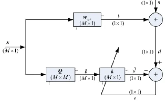
In Fig. 1, the input signal vector , optimal coefficient vector , orthogonal input vector
and regression coefficient are vectors. And is an
× orthogonal transform matrix.
+
Q b +
x
n
d ˆd
opt y w
e (M×1)
(M×1) (1 1)× (1 1)×
(1 1)×
(M M× ) (M×1) (Mk×1) (1 1)× (1 1)×
+ -
그림 1. 직교입력벡터를 이용한 적응 필터의 구조
Fig. 1. The structure of an adaptive filter using an orthogonal input vector.
The signal is the desired response, is the estimated desired response and is the measurement noise. As shown in Fig. 1, the system is excited by an input signal , and we are looking for the estimated values of the, the unknown tap coefficients.
That is,
* 2
[ ( ) ( )] [| ( ) | ]
J =E e n e n =E e n (1)
is a minimum.
The error is defined as following
( ) ( ) H ( )
e n =d n − k b n (2)
where, (H)is a Hermitian transpose. and
are expressed as follows
ˆ( ) H ( ) H ( )
d n =k b n =k Qx n (3)
( )n = ( )n
b Qx (4)
And we define the desired response as
( ) optH ( )
d n = w x n (5)
The error reaches zero if is equal to
. That is,
( ) ˆ( ) [ optH H ] ( ) 0
d n −d n = w −k Q x n = (6) If x( ) 0n ≠ , the solution of the above equation becomes
H opt =
w Q k (7)
Generally, if the orthogonal input vector is used, the regression coefficient and the coefficient of the TDL filter are related to each other, as presented in (7).
Using (1), the gradient of the mean-squared error can be obtained as following
2 [( ( ) H ( ))( H( ))]
J E d n n n
∂ = − −
∂ k b b
k (8)
From the above equation, the vector can be represented as
1 *
[ ( ) H( )] [ ( ) ( )]
E n n − E n d n
=
k b b b (9)
Rewriting the above equation using a matrix form, we obtain.
1 bb bd
= −
k R p (10)
[ ( ) H( )]
bb =E n n
R b b (11)
[ ( ) ( )]* bd =E n d n
p b (12)
Where is an autocorrelation matrix of , We have to assume that is a nonsingular matrix. In this paper, we proposed the theorem that can determine
directly without any calculation of .
Theorem 1. If the desired response and the estimated desired response have so similar values, the relationship R wbx opt = pbd is defined.
proof)
Substituting (4) and (7) into (8), we get 2 [( ( ) optH 1 ( ))( H( ))]
J E d n − n n
∂ = − −
∂ w Q Qx b
k (13)
The optimal coefficient can be obtained from (13) using Q Q−1 =I .
[ ( ) H( )] opt [ ( ) ( )]*
Eb n x n w =Eb n d n (14)
The equation (14) can be simplified as
bx opt = bd
R w p (15)
where
[ ( ) H( )]
bx =E n n
R b x (16)
Q.E.D.
The matrix in (16) is the correlation matrix of the orthogonal input vector and nonorthogonal input vector , and is nonsingular[1].
Ⅲ. Computer Simulation
To evaluate the performance of the proposed algorithm, the identification of an unknown FIR system is performed. The input signal x n( ) to the adaptive filter was obtained from the output of a low pass filter which transfer function is as follows;
1 2 3 4 5
( ) 1
1 0.98 0.693 0.22 0.309 0.177
H z = z− z− z− z− z−
− + − + −
(17) where, its input is a white, zero mean and pseudorandom Gaussian noise. The response signal
was obtained from the FIR system, as shown in (18).
1 2 3
( ) 2.65 3.31 2.24 0.7
H z = − z− + z− − z− (18) The measurement noise signal was an additive white, zero mean and pseudorandom Gaussian and was uncorrelated with the input signal. The computer simulation is designed to determine the similarities of the coefficient of the filters by solving the Wiener-Hopf equation and the equivalent Wiener-Hopf equation. All
results presented in this paper are ensemble averages of 100 independent runs with 9000 data. Fig. 2 shows that the curves of the (w( )xxi −wopt( )i ) /wopt( )i ,
( ) ( ) ( )
(wbxi −wopti ) /wopti and (wbs( )i −w( )opti ) /w( )opti obtained from the solutions of the Wiener-Hopf and equivalent Wiener-Hopf equation for an SNR of -90dB, -30dB, -10dB and 10dB, respectively. is the i-th optimal coefficient, is the i-th solution of original Wiener-Hopf equation and is the i-th solution of the proposed equivalent Wiener-Hopf equation.
(a)
(b)
그림 2. 상관행렬의 변화에 따른 계수 비교
(a) 미지시스템 차수 : 20, 시스템식별차수 : 20 (b) 미지시스템 차수 : 20, 시스템식별차수 : 10 Fig. 2. Comparison of coefficients according to
variation of correlation matrix.
(a) order of unknown system; 20, order of system identification; 20.
(b) order of unknown system;20, order of system identification; 10.
The following simulation is made when the rank is deficient. Fig. 2 illustrates the results obtained by varying the rank of autocorrelation.
In Fig. 2, we set an order of unknown system to 20 and one of computer simulation to 10 under SNR of -30dB, respectively.
Fig. 2 shows the results of the coefficients for various ranks of the correlation matrix. The matrix is full rank. The figure shows that both the existing method and the proposed method have similar performance. Fig. 2 (b) is the case of a rank deficiency.
This figure shows the simulation results of an unknown system of order 20, while the order of the simulated adaptive filter is 10. The figure shows that the proposed method and existing method produce similar results.
Ⅳ. Conclusion
In this paper, an equivalent Wiener-Hopf equation is proposed. The proposed algorithm can determine the coefficient of a TDL filter directly when the adaptive filter has an orthogonal input signal. Also, a theoretical analysis was performed for the MMSE using a solution to the equivalent Wiener-Hopf equation. Furthermore, the proposed algorithm shows similar performance to that of the original Wiener-Hopf equation.
The proposed algorithm has the advantage of allowing the application area of adaptation filters which have an orthogonal input signal to be expanded.
References
[1] Haykin, Adaptive Filter Theory–Fourth Edition, PrenticeHall.
[2] J. G. Proakis, C. M. Rader, F. Ling and C. L.
Nikias, Advanced Digital Signal Processing.
Macmillan Publishing Company,1992.
[3] P. S. R. Diniz, Adaptive Filtering -Algorithms
and Practical Implementation, second edition.
Kluwer Academic Publishers, 2002.
[4] J. Makhoul. "A Class of ALL-Zero Lattice Digital Filters: Properties" IEEE Trans. Acoustics, Speech, and Signal Processing, vol. ASSP-26, pp.304-314, Aug. 1978.
[5] E. Karlsson, M. Hayes, “Least squares ARMA modeling of linear time-varying systems: Lattice filter structures and fast RLS algorithms,” IEEE Trans. Acoustics, Speech, and Signal Processing, vol.ASSP-35, NO.7, pp.994-1014, July1987.
[6] H. K. Baik, V. J. Mathews, “Adaptive lattice bilinear filters,” IEEE Trans. on Signal Processing, vol.41, pp.2033-2046, June1993.
[7] L. Fuyun, J. Proakis, "A generalized multichannel least squares lattice algorithm based on sequential processing stages," IEEE Trans. on Signal Processing, vol.32, pp.381-389, Apr.1984.
저자 소개
조 주 필(정회원)
∙2001년: 전북대학교 전자공학과 공학 박사
∙2000년~2005년:한국전자통신연구원 이동통신연구단 선임연구원
∙2006년~2007년: ETRI 초빙연구원
∙2011년~:미국 University of South Florida, Visiting Researcher
∙2005년~ 현재 : 군산대학교 공과대학 전파공학과 부교수
<주관심분야 : Cognitive-Radio, 주파수 융합기술, LTE >
차 재 상(정회원)
∙2000년: 일본 東北(Tohoku)대학교 전자 공학과(공학박사)
∙2000년~2002년: 한국전자통신연구원 (ETRI) 무선방송 기술연구소 선임연구원
∙2002년~2005년: 서경대학교 정보통신공 학과 전임강사
∙2008년: 미국 Florida University, Visiting Professor
∙2005년~ 현재 : 서울과학기술대학교 매체공학과 부교수
<주관심분야 : LED-ID, 조명IT융합신기술, LBS, ITS, UWB, 무선홈네트워크, DMB 및 디지털 방송 등>
이 일 규(정회원)
∙2003년: 충남대학교 전자공학과 공학 박사
∙1997년~2004년:한국전자통신연구원 (ETRI) 선임연구원
∙2004년~현재 : 공주대학교 전기전자 제어공학부 부교수
<주관심분야 : RF 부품 및 시스템, 안테나 및 전파 전파, 전 파 간섭>