Development and Positioning Accuracy Assessment of Precise Point Positioning Algorithms Based on GLONASS Code-Pseudorange Measurements

JPNT 3(4), 155-161 (2014)

http://dx.doi.org/10.11003/JPNT.2014.3.4.155

Copyright © The Korean GNSS Society

J ^PNT

Journal of Positioning, Navigation, and Timing

http://www.gnss.or.kr Print ISSN: 2288-8187 Online ISSN: 2289-0866

1. INTRODUCTION

The market for location information services is expanding worldwide, and many Global Navigation Satellite System (GNSS) services are being developed to satisfy the needs of users who demand accurate location information in various fields (Kim 2013). Precise point positioning (PPP) is the most appropriate technology to apply to portable navigation of users since it has similar performance with Differential GPS (DGPS) without installing a separate device or reference station, as precise positioning is carried out solely by the receiver at the observing point. However, if PPP is conducted using only GPS, it has the limitation of not being able to calculate the location of the user when the visibility of satellite is not sufficiently secured. If GLObal NAvigation Satellite System (GLONASS), which succeeded

Development and Positioning Accuracy Assessment of Precise Point Positioning Algorithms Based on GLONASS Code-Pseudorange

Measurements

Mi-So Kim

¹

, Kwan-Dong Park

^1†

, Jihye Won

²

1

Department of Geoinformatic Engineering, Inha University, Incheon 402-751, Korea

2

Jipyong Space Inc., Incheon 402-751, Korea

ABSTRACT

The purpose of this study is to develop precise point positioning (PPP) algorithms based on GLONASS code-pseudorange, verify their performance and present their utility. As the basic correction models of PPP, we applied Inter Frequency Bias (IFB), relativistic effect, satellite antenna phase center offset, and satellite orbit and satellite clock errors, ionospheric errors, and tropospheric errors that must be provided on a real-time basis. The satellite orbit and satellite clock errors provided by Information-Analytical Centre (IAC) are interpolated at each observation epoch by applying the Lagrange polynomial method and linear interpolation method. We applied Global Ionosphere Maps (GIM) provided by International GNSS Service (IGS) for ionospheric errors, and increased the positioning accuracy by applying the true value calculated with GIPSY for tropospheric errors. As a result of testing the developed GLONASS PPP algorithms for four days, the horizontal error was approximately 1.4

~ 1.5 m and the vertical error was approximately 2.5 ~ 2.8 m, showing that the accuracy is similar to that of GPS PPP.

Keywords: GLONASS, precise point positioning, code pseudo range, phase center offset

in system normalization in 2011, is used to supplement the aforementioned limitation, the user’s location cannot be calculated without securing the visibility of GPS satellite.

The basic concept of PPP was introduced by Malys &

Ortiz (1989), and since Héroux & Kouba (1995) used the term “PPP” for the first time, various studies have been conducted until recently. Witchayangkoon (2000) studied PPP algorithms using satellite orbit and satellite clock error correction information provided by International GNSS Service (IGS, http://igscb.jpl.nass.gov/index.

html), and Gao & Chen (2004) studied PPP algorithms applying satellite orbit and satellite clock error correction information on a real-time basis. A study on PPP using GLONASS is conducted by Defraigne & Baire (2011), who matched the hour meter of the GLONASS system with the GPS system and studied the method to determine the frequency of GLONASS satellites with different frequencies using channel numbers provided by broadcast ephemeris and apply to PPP. Cai & Gao (2013) conducted PPP by studying the hardware errors that occur by the frequency division system of GLONASS. In Korea, Choi et al. (2011) developed PPP algorithms and calculated location Received Oct 08, 2014 Revised Nov 17, 2014 Accepted Nov 20, 2014

†

Corresponding Author E-mail: [email protected]

Tel: +82-32-860-7604 Fax: +82-32-863-1506

http://dx.doi.org/10.11003/JPNT.2014.3.4.155

information with approximately 3 cm of error level for static positioning, and Ha et al. (2012) analyzed the accuracy of PPP using predicted ephemeris of GIPSY. The previous studies mentioned above have limitations in applying to the portable navigations of users since the focus is on PPP based on carrier-phase observed value. Moreover, previous studies on PPP using GLONASS observed value are mostly about converting the hour meter of the GLONASS system and applying errors by the frequency division system. Thus, it is necessary to conduct additional research on correction of errors such as ionospheric errors or tropospheric errors.

This study is a prestudy to develop GPS/GLONASS integrated PPP algorithms, and it developed PPP algorithms using observed values of GLONASS code-pseudorange.

We aimed to analyze the performance according to the application of the error model of PPP algorithms developed in this study by applying the satellite orbit and satellite clock error correction information provided by Information- Analytical Centre (IAC, http://glonass-iac.ru/en/) and using the Global Ionosphere Maps (GIM) provided by IGS and tropospheric correction information calculated with GNSS Inferred Positioning System and Orbit Analysis Simulation Software package (GIPSY-OASIS).

2. GLONASS ERROR CORRECTION MODEL FOR PPP

The observed value of code-pseudorange is determined by using the signal transmission time for the distance between the satellite and receiver. However, while hardware errors and signals of the satellite and receiver are transmitted, the atmospheric impacts on signals hinder accurate positioning.

The observation equation of code-pseudorange including each error factor is as shown in Eq. (1). In Eq. (1), δt

_r

is receiver clock error, δt

^s

is satellite clock error, δI is ionospheric delay error, δT is tropospheric delay error, δM is multipath error, δ

_r

is receiver hardware error, δ

^s

is satellite hardware error, and ε is probable error (Misra & Enge 2011).

p    c t ⁽ 

r

  t

^s

⁾     I T   M      

r ^s

4.4428076333 10

10

sin

t

RL ^

e a E

   

1 (

2

)

RL x y z

t xv yv zv

  c  

_ 1

(1602 0.5625)

Glonass L

f   FCN  MHz

_ 2

(1246 0.4375)

Glonass L

f   FCN  MHz

16

2 6 2

40.3 40.3 10

( 10 )

Glonass Glonass

Total number of electrons

I TECU TEC

Frequency f f



   ^



( ) ( )

h w h w

T T T m el ZHD m el ZWD

      

ZTD AHD AWD ZDC

  

(2.2779 0.0024) P

s

ZHD  

(1)

To increase accuracy of PPP, the correction process of error factors is essential. However, for code-pseudorange used in this study, the size of the noise is ~m, indicating that there are error factors with very small impacts on positional accuracy improvement due to correction. Therefore, this study excluded error factors with small impacts on accuracy improvement and divided the remaining factors into two categories. The first category includes Inter Frequency Bias

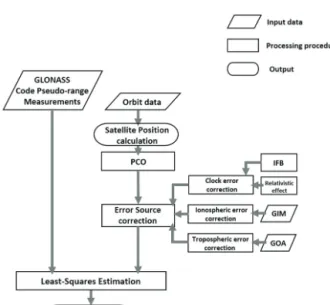
(IFB), relativistic effect, and phase center offset (PCO) errors that must be basically considered, and the second category includes GLONASS satellite orbit that must be applied as real-time correction information as well as clock error, ionospheric error and tropospheric error. The application process of correction information of PPP algorithms developed in this study is as shown in Fig. 1.

2.1 Basic Model

2.1.1 IFB and Relativistic Effects

IFB is errors on the hardware of satellite and receiver that occur in the process in which the frequency processes other signals. IFB occurs in all codes and carrier signals, and has different values according to the type of satellite and receiver. The IFB of code signals is also referred to as Differential Code Bias (DCB) (Kim 2013).

Unlike GPS, the signal division system of GLONASS is the Frequency Division Multiple Access (FDMA) method in which observed values have different frequencies for each satellite, which affects IFB. Therefore, IFB must be considered in PPP using GLONASS code-pseudorange (Aggrey & Bisnath 2014). The header part of IONosphere EXchange (IONEX) file provided by IGS provides DCB value of GLONASS and GPS, and this study calculated the correction quantity of IFB using the DCB value of IONEX file and frequency ratio of satellite signals.

The relativistic effects occur differently according to the relative motions of the satellite and receiver. They also influence the satellite orbit and signal transmission

Fig. 1. Flowchart of PPP algorithms process.

Mi-So Kim et al. Precise Point Positioning based on GLONASS 157

http://www.gnss.or.kr path and generate various errors on the clocks of satellites

and receivers. This study considered only the impacts of relativistic effects on satellite clock errors. The relativistic effects of GPS satellite are corrected by applying satellite eccentricity (e) provided by GPS broadcast ephemeris, semi- major axis (a), and eccentric anomaly (E) to Eq. (2) (Misra

& Enge 2011). However, it is easier to correct the relativistic effects of GLONASS satellite by applying the location and speed of satellite provided by GLONASS broadcast ephemeris to Eq. (3) (Xu 2007). Therefore, this study used Eq. (3) to correct the relativistic effects.

(

r ^s

)

r ^s

p    c t    t     I T   M      

4.4428076333 10

10

sin

t

RL ^

e a E

   

1 (

2

)

RL x y z

t xv yv zv

  c  

_ 1

(1602 0.5625)

Glonass L

f   FCN  MHz

_ 2

(1246 0.4375)

Glonass L

f   FCN  MHz

16

2 6 2

40.3 40.3 10

( 10 )

Glonass Glonass

Total number of electrons

I TECU TEC

Frequency f f



   ^



( ) ( )

h w h w

T T T m el ZHD m el ZWD

      

ZTD AHD AWD ZDC

  

(2.2779 0.0024) 1 0.00266cos2 0.00028

P

s

ZHD  h

 

 

(2)

(

r ^s

)

r ^s

p    c t    t     I T   M      

4.4428076333 10

10

sin

t

RL ^

e a E

   

1 (

2

)

RL x y z

t c xv yv zv

   

_ 1

(1602 0.5625)

Glonass L

f   FCN  MHz

_ 2

(1246 0.4375)

Glonass L

f   FCN  MHz

16

2 6 2

40.3 40.3 10

( 10 )

Glonass Glonass

Total number of electrons

I TECU TEC

Frequency f f



   ^



( ) ( )

h w h w

T T T m el ZHD m el ZWD

      

ZTD AHD AWD ZDC

  

(2.2779 0.0024) 1 0.00266cos2 0.00028

P

s

ZHD  h

 

 

(3)

In Eq. (2), e is orbital eccentricity, a is semi-major axis, and E is eccentric anomaly; in Eq. (3), c is speed of light, and (x, y, z) and (v

_x

, v

_y

, v

_z

) are satellite location and speed on the ECEF coordinate system.

2.1.2 Phase Center Offset

The observed value of code-pseudorange which is the distance between the satellite and receiver is provided as the phase center of transmitter/receiver antenna, and the orbit information coordinate of precise ephemeris is provided as the mass center of the satellite. The phase center and mass center of the satellite do not match with each other, and thus we need the process of converting the mass center coordinate of orbit information into the phase center coordinate in order to obtain more precise positioning result (Xu 2007).

Phase center variation (PCV) indicates the variance of mass center and phase center of antenna, and has different values according to frequency, antenna and satellite.

The mean value of PCV is phase center offset (PCO), and IGS provides phase center offset information of GPS and GLONASS in the form of ANTenna Exchange Format (ANTEX). PCV must be applied in precise positioning using the carrier-phase observed value, but just applying phase center offset is enough for precise positioning using the code-pseudorange observed value (Misra &

Enge 2011). In this study, we corrected the phase center offset by calculating the unit vector and rotation matrix in satellite body fixed reference frame using the IGS08 version information provided by ANTEX file.

2.2 Correction Information

2.2.1 Satellite Orbit and Satellite Clock Errors

To determine the coordinate of the receiver, we need the coordinate value of the satellite aside from the code- pseudorange observed value, and the coordinate of the satellite can be determined through the calculation using broadcast ephemeris or interpolation of precise ephemeris.

This study converted the coordinate into that of satellite observation time by applying the Lagrange polynomial that is optimum for precise ephemeris at 15-minute intervals provided by IAC (Kim 2009).

For satellite clock errors, there is the method of using the correction information at 30-minute intervals provided through broadcast ephemeris or correction information at 15-minute intervals provided through precise ephemeris, but this study used the clock error correction information provided by IAC in the form of CLK file. To use the CLK file that provides satellite clock error information at 5-minute or 30-second intervals, it is necessary to convert to the error value of observation time.

Since satellite clock errors are not significantly influenced by interpolation, the data processing speed was increased using the linear interpolation (Guo et al. 2010).

2.2.2 Ionospheric Errors

Ionosphere is made up of electrons and ions, among which electrons are easily influenced by external factors and thus distort and delay signals by colliding with them when satellite signals pass through the atmosphere. When observing dual frequency, ionospheric errors can be completely eliminated with ionospheric-free combination;

however, for single frequency, correction of ionospheric

errors is essential (Park et al. 2014). A general method to

correct ionospheric errors is to use the Klobuchar model,

which is a GPS ionospheric correction model, or the

NeQuick model, which is a Galileo ionospheric correction

model, as well as GIM model provided by IGS. In the case

of GLONASS, ionospheric correction factors to use the

Klobuchar and NeQuick model are not provided, but it

is possible to apply the Klobuchar and NeQuick models

to the correction of GLONASS ionospheric errors by

using the ratio of inter-satellite frequency. However, this

method can eliminate only about 50 ~ 60% of ionospheric

errors (Klobuchar 1987). Therefore, this study corrected

ionospheric errors using the GIM provided by IGS. The

GIM divides the globe into 2.5˚ × 5.0˚ grids and provides

the total number of ionosphere electrons in IONEX files at

2-hour intervals. The total number of electrons is provided

158 JPNT 3(4), 155-161 (2014)

as information on vertical direction under the assumption that electrons are concentrated on the single layer with the thickness of 0 at the altitude of 450km, and thus it is necessary to convert this to error in the gaze direction.

The unit of the number of electrons is TECU, and 1TECU indicates a distribution of 1 × 10

¹⁶

free electrons on 1 m

²

unit area.

Ionospheric correction quantity varies according to the satellite frequency as well as the atmospheric condition.

GPS has different frequencies for each signal with the code division multiple access (CDMA), but GLONASS has different frequencies for each satellite with the FDMA.

Therefore, for ionospheric correction of GLONASS, the process of calculating the frequency of each satellite is essential. The frequency of GLONASS satellite is determined by the channel numbers provided in the navigation message as shown in Eqs. (4) and (5), and the calculated frequency of satellite is applied to Eq. (6) to calculate the ionospheric delay.

(

r ^s

)

r ^s

p    c t    t     I T   M      

4.4428076333 10

10

sin

t

RL ^

e a E

   

1 (

2

)

RL x y z

t xv yv zv

  c  

_ 1

(1602 0.5625)

Glonass L

f   FCN  MHz

_ 2

(1246 0.4375)

Glonass L

f   FCN  MHz

16

2 6 2

40.3 40.3 10

( 10 )

Glonass Glonass

Total number of electrons

I TECU TEC

Frequency f f



   ^



( ) ( )

h w h w

T T T m el ZHD m el ZWD

      

ZTD AHD AWD ZDC

  

(2.2779 0.0024) 1 0.00266cos2 0.00028

P

s

ZHD  h

 

 

(4)

(

r ^s

)

r ^s

p    c t    t     I T   M      

4.4428076333 10

10

sin

t

RL ^

e a E

   

1 (

2

)

RL x y z

t xv yv zv

  c  

_ 1

(1602 0.5625)

Glonass L

f   FCN  MHz

_ 2

(1246 0.4375)

Glonass L

f   FCN  MHz

16

2 6 2

40.3 40.3 10

( 10 )

Glonass Glonass

Total number of electrons

I TECU TEC

Frequency f f



   ^



( ) ( )

h w h w

T T T m el ZHD m el ZWD

      

ZTD AHD AWD ZDC

  

(2.2779 0.0024) 1 0.00266cos2 0.00028

P

s

ZHD  h

 

 

(5)

(

r ^s

)

r ^s

p    c t    t     I T   M      

4.4428076333 10

10

sin

t

RL ^

e a E

   

1 (

2

)

RL x y z

t xv yv zv

  c  

_ 1

(1602 0.5625)

Glonass L

f   FCN  MHz

_ 2

(1246 0.4375)

Glonass L

f   FCN  MHz

16

2 6 2

40.3 40.3 10

( 10 )

Glonass Glonass

Total number of electrons

I TECU TEC

Frequency f f



   ^



( ) ( )

h w h w

T T T m el ZHD m el ZWD

      

ZTD AHD AWD ZDC

  

(2.2779 0.0024) 1 0.00266cos2 0.00028

P

s

ZHD  h

 

 

(6)

In Eqs. (4) and (5), Frequency Channel Number (FCN) indicates channel number; and in Eq. (6), f

Glonass

indicates the frequency of satellite determined by Eqs. (4) or (5).

2.2.3 Tropospheric Errors

When the signals of the satellite pass through the atmosphere, they are distorted and delayed by dry air and vapor in the troposphere. The degree of tropospheric errors is determined by temperature, humidity and atmospheric pressure, and the refractive index is the same regardless of frequency and thus cannot be eliminated even by using dual frequency. Therefore, to eliminate tropospheric errors, it is necessary to use statistical estimation or empirical model (Park et al. 2014).

Zenith Hydrostatic Delay (ZHD) that takes up 90% of tropospheric errors has physically stable distribution and can be accurately corrected by using pressure. However, Zenith Wet Delay (ZWD) that takes up 10% of tropospheric errors has big changes according to weather conditions and thus cannot be accurately corrected (Kim 2013). The tropospheric error of two types of delay is presented as shown in Eq. (7).

4.4428076333 10

10

sin

t

RL ^

e a E

   

1 (

2

)

RL x y z

t xv yv zv

  c  

_ 1

(1602 0.5625)

Glonass L

f   FCN  MHz

_ 2

(1246 0.4375)

Glonass L

f   FCN  MHz

16

2 6 2

40.3 40.3 10

( 10 )

Glonass Glonass

Total number of electrons

I TECU TEC

Frequency f f



   ^



( ) ( )

h w h w

T T T m el ZHD m el ZWD

      

ZTD AHD AWD ZDC

  

(2.2779 0.0024) 1 0.00266cos2 0.00028

P

s

ZHD  h

 

 

(7) In Eq. (7), δT is the tropospheric error of the gaze direction, and this value is equivalent to the sum of δT

_h

, the ZHD of the gaze direction, and δT

_w

, the ZWD of the gaze direction. The ZHD and ZWD of the gaze direction can be calculated by applying the altitude el, dry mapping function m

_h

, and wet mapping function m

_w

to the ZHD and ZWD of the zenith direction. The mapping function is a function that converts the delay of the zenith direction into delay of the gaze direction in which the signal is transmitted from the satellite to the receiver (Won et al. 2010).

This study compared the degree of improvement according to the tropospheric error correction model by applying the GIPSY calculation method (GOA) and Global Pressure and Temperature (GPT). GOA is the method of calculating total tropospheric delay by adding up the values of A priori Hydrostatic Delay (AHD) and A priori Wet Delay (AWD) as well as Zenith Delay Correction (ZDC) of the a priori delay estimated in GIPSY. This process is as shown in Eq. (8) (Kim et al. 2012).

(

_r ^s

)

_r ^s

p    c t    t     I T   M      

4.4428076333 10

10

sin

t

RL ^

e a E

   

1 (

2

)

RL x y z

t xv yv zv

  c  

_ 1

(1602 0.5625)

Glonass L

f   FCN  MHz

_ 2

(1246 0.4375)

Glonass L

f   FCN  MHz

16

2 6 2

40.3 40.3 10

( 10 )

Glonass Glonass

Total number of electrons

I TECU TEC

Frequency f f



   ^



( ) ( )

h w h w

T T T m el ZHD m el ZWD

      

ZTD AHD AWD ZDC

  

(2.2779 0.0024) 1 0.00266cos2 0.00028

P

s

ZHD  h

 

 

(8)

Total tropospheric delay is equal to the sum of ZHD and ZWD, and ZHD can be calculated with Eq. (9). In Eq.

(9), φ is the latitude of the observatory, h is the ellipsoid of the observatory [m], and P

_s

is the atmospheric pressure acquired from meteorological sensor (Elgered et al. 1991).

We calculated the difference between the total tropospheric delay calculated from Eq. (8) and the ZHD value obtained from Eq. (9) to quantitatively divide ZHD and ZWD. We corrected the tropospheric error toward the gaze direction by applying Global Mapping Function (GMF) to the estimated ZHD and ZWD. GMF has similar accuracy with Vienna Mapping Function (VMF) and can be applied on a real-time basis unlike VMF, and it is a mapping function expanded so that the regionally limited data of VMF can be used in all global scope (Kim 2013).

(

r ^s

)

r ^s

p    c t    t     I T   M      

4.4428076333 10

10

sin

t

RL ^

e a E

   

1 (

2

)

RL x y z

t xv yv zv

  c  

_ 1

(1602 0.5625)

Glonass L

f   FCN  MHz

_ 2

(1246 0.4375)

Glonass L

f   FCN  MHz

16

2 6 2

40.3 40.3 10

( 10 )

Glonass Glonass

Total number of electrons

I TECU TEC

Frequency f f



   ^



( ) ( )

h w h w

T T T m el ZHD m el ZWD

      

ZTD AHD AWD ZDC

  

(2.2779 0.0024) 1 0.00266cos2 0.00028

P

s

ZHD  h

 

  (9)

GPT is an empirical model based on spherical harmonic function providing atmospheric pressure and temperature all over the globe. If latitude, altitude and observation date of the observatory are entered, it calculates the relevant atmospheric pressure and temperature (Böhm et al. 2012).

ZHD can be calculated by applying the latitude ( φ ) and

altitude (h) of the observatory and atmospheric pressure (P

_s

)

Mi-So Kim et al. Precise Point Positioning based on GLONASS 159

http://www.gnss.or.kr calculated from the GPT model to Eq. (9). The calculated

ZHD is corrected with gaze direction error by applying simple mapping function to the altitude angle. Parts relevant to ZWD are not considered in the GPT method.

3. PPP PERFORMANCE EVALUATION OF GLONASS

3.1 Observation Data

For performance verification and utility evaluation according to the application of PPP algorithms based on GLONASS code-pseudorange developed in this study to correction information, we used the IHUR observatory located in Inha University. IHUR uses the NetR5 receiver by Trimble and TRM41249.00 antenna, and we used the data recorded at 30-second intervals on July 31, 2014 (DOY212) and August 9 (DOY221), 19 (DOY231), and 29 (DOY241), 2014. Moreover, we collected pressure data through the meteorological sensor of Paroscientific Met-4A and divided tropospheric errors into ZHD and ZWD. We verified the performance of PPP algorithms on the basis of precise coordinate of IHUR observatory calculated with GIPSY.

3.2 Positioning Performance Evaluation Result According to the Application of Error Models

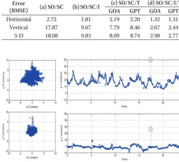
We evaluated the positioning performance according to the application of error models by applying the aforementioned error factors. Moreover, to determine the positioning performance according to the application of atmospheric correction information, we applied the correction of the basic model and clock error, after which we applied the correction of ionospheric errors and tropospheric errors in order. We applied the GIM model for ionospheric error correction, and GOA and GPT model for tropospheric error correction, comparing the degree of improvement in positioning accuracy. Table 1 is a result of applying each error correction model to the data of July 31, 2014 (DOY: 212). (a) is the case in which satellite orbit (SO) and satellite clock (SC) error correction models are applied; (b) is the case in which ionosphere (I) correction model is applied to (a); (c) is the case in which troposphere (T) correction model is applied to (a); and (d) is the case in which both ionosphere and tropospheric errors are applied to (a).

Table 1 shows that the accuracy improvement in the vertical direction is greater than in horizontal direction for both when ionospheric errors and tropospheric errors are corrected. An additional characteristic is that ionospheric

error correction improves horizontal accuracy more than tropospheric error correction, while tropospheric error correction improves vertical accuracy more than ionospheric error correction. As a result of verifying the contribution level of positioning accuracy improvement of the atmospheric model by applying both ionospheric and tropospheric error correction, it was found that, when GOA is applied, horizontal error is improved by approximately 51.4% from 2.72 m to 1.32 m and vertical error by 85% from 17.87 m to 2.67 m, compared to the case in which only satellite orbit error and satellite clock error are applied. This improvement can be found in Fig. 2 as well. Moreover, Fig. 2 also shows the increase in errors in certain sections, which is due to the temporary increase in errors in sections where visibility of satellite is not sufficiently secured.

To determine the performance of developed algorithms, we additionally tested 3 days (DOY: 221, 231, 241) aside from July 31, 2014 (DOY 212). Table 2 shows the result of (d) in which satellite orbit, satellite clock errors, ionospheric errors and tropospheric errors are all applied to four days.

1-1) Horizontal coordinate error of (a) SO/SC 1-2) Vertical coordinate error of (a) SO/SC 2-1) Horizontal coordinate error of (d) SO/SC/I/T 2-2) Vertical coordinate error of (d) SO/SC/I/T

Fig. 2. Horizontal and vertical PPP positioning error.

Table1. Positioning accuracy according to the application of each error correction model (unit: m)..

Error

(RMSE) (a) SO/SC (b) SO/SC/I (c) SO/SC/T (d) SO/SC/I/T GOA GPT GOA GPT

Horizontal 2.72 1.81 2.19 2.20 1.32 1.31

Vertical 17.87 9.67 7.79 8.46 2.67 2.44

3-D 18.08 9.83 8.09 8.74 2.98 2.77

Table 2. Positioning accuracy according to the application of data per date (unit: m).

Error (RMSE)

DOY 212 DOY 221 DOY 231 DOY 241 Average GOA GPT GOA GPT GOA GPT GOA GPT GOA GPT Horizontal 1.32 1.31 1.6 1.6 1.42 1.42 1.51 1.51 1.46 1.46 Vertical 2.67 2.44 2.67 2.35 2.92 2.68 2.84 2.54 2.75 2.5 3-D 2.98 2.77 3.12 2.84 3.25 3.03 3.22 2.96 3.14 2.9

As a result of the four-day testing, it was found that it would be possible to carry out positioning with the error of 1.4

~ 1.5 m horizontally and 2.5 ~ 2.8 m vertically if accurate correction information is provided for PPP algorithms based on GLONASS code-pseudorange developed in this study. A comparison of the result of applying GOA and GPT to tropospheric correction model, it was found that the case in which GOA was applied showed accuracy that is approximately 20 ~ 30 cm higher in the vertical direction than when GPT is applied. This phenomenon occurs when both ionospheric correction and tropospheric correction are applied simultaneously. When only tropospheric correction information is applied, GOA showed higher positioning accuracy (see Table 1). Since tropospheric correction information has more influence on vertical error than horizontal error, vertical error varied according to the tropospheric correction model. However, when ionospheric correction and tropospheric correction are applied simultaneously, the result of applying GOA has lower accuracy than GPT, regarding which there is a need for additional research to determine the cause.

4. CONCLUSION

When positioning was carried out using only GPS satellite, there was the limitation in which the user cannot obtain the location when the visibility of the satellite is not sufficiently secured. As a prestudy of GPS/GLONASS integrated PPP development, we developed PPP algorithms using the observed values of GLONASS code-pseudorange and verified the performance. For accurate positioning, we used precise ephemeris of IAC for satellite orbit and satellite clock errors, and applied Lagrange and linear interpolation algorithms to calculate the optimum value of the relevant positioning vision. Moreover, we corrected IFB and relativistic effects that must be considered since they are not eliminated in the single positioning, and applied phase center offset per satellite. We applied the GIM model provided by IGS for ionospheric error correction, and applied the true value calculated with GIPSY and the empirical model GPT based on spherical harmonic function for tropospheric error correction, and compared the results.

As a result of conducting a test for four days to evaluate the performance of PPP algorithms developed in this study, it was found that horizontal error was 1.4 ~ 1.5 m and vertical error was 2.5 ~ 2.8 m. This result is similar to the accuracy of 1 ~ 2 m obtained by Kim (2013) and Park et al. (2014) after conducting PPP using the observed values of GPS code- pseudorange, thereby proving the utility of the algorithms

developed in this study. If follow-up research establishes the environment to develop GPS/GLONASS integrated PPP and provide real-time correction information, the utilization of PPP algorithms based on GLONASS code-pseudorange developed in this study is expected to increase.

ACKNOWLEDGMENTS

T h i s re s e a rc h w a s s u p p o r t e d b y a g r a n t f ro m

“Development of GNSS based Transportation Infrastructure Technology” funded by Ministry of Land, Infrastructure and Transport of Korean government.

REFERENCES

Aggrey, J. & Bisnath, S. 2014, Analysis and Modelling of Pseudorange and Carrier-phase Biases in GNSS Precise Point Positioning, in 2014 ION GNSS+, Tampa, Florida, USA, 8-12 Sep. 2014

Böhm, J., Lagler, K., Schindelegger, M., Krásná, H., & Nilsson, T. 2012, GPT2/GMF2: An improved empirical model for troposphere delays, in 2012 AGU Fall Meeting, San Francisco, USA, 3-7 Dec 2012

Cai, C. & Gao, Y. 2013, GLONASS-Based Precise Point Positioning and Performance Analysis, Advances in Space Research, 51, 514-524. http://dx.doi.org/10.1016/

j.asr.2012.08.004

Choi, B. K., Back, J.-H., Cho, S.-K., Park, J.-U., & Park, P.- H. 2011, Development of precise point positioning method using global positioning system measurements, JASS, 28, 217-223. http://dx .doi.org/10.5140/

JASS.2011.28.3.217

Defraigne, P. & Baire, Q. 2011, Combining GPS and GLONASS for Time and Frequency transfer, Advances in Space Research, 47, 265-275. http://dx.doi.

org/10.1016/j.asr.2010.07.003

Elgered, G., Davis, J. L., Herring, T. A., & Shapiro, I. I.

1991, Geodesy by Radio Interferometry: Water Vapor Radiometry for Estimation of the Wet Delay, JGR, 96, 6541-6555. http://dx.doi.org/10.1029/90JB00834 Gao, Y. & Chen, K. 2004, Performance Analysis of Precise Point

Positioning using Real-time Orbit and Clock products, Journal of Global Positioning Systems, 3, 95-100

Guo, F., Zhang, X., Li, X., & Cai, S. 2010, Impact of Sampling Rate of IGS Satellite Clock on Precise Point Positioning, Geo-spatial inform. Sci, 13, 150-156. http://dx.doi.

org/10.1007/s11806-010-0226-9

Ha, J-H., Heo, M-B., & Nam, G-W. 2012, Accuracy Analysis of

Mi-So Kim et al. Precise Point Positioning based on GLONASS 161

http://www.gnss.or.kr Precise Point Positioning Using Predicted GPS Satellite

Orbits, The Journal of Korea Navigation Institute, 16, 752-759

Héroux, P. & Kouba, J. 1995, GPS Precise Point Positioning with A Difference, Geomatics ’95, Ottawa, Ontario, Canada, June 13-15, 1995

Klobuchar, J. A. 1987, Ionospheric time-delay algorithm for single-frequency GPS users, IEEE Trans Aerosp Electron Syst, AES-23, 325-331. http://dx.doi.org/10.1109/

TAES.1987.310829

Kim, D., Won, J., Son, E.-S., & Park, K.-D. 2012, Generation of Grid Maps of GPS Signal Delays in the Troposphere and Analysis of Relative Point Positioning Accuracy Enhancement, Journal of Korean navigation and port research, 36, 825-832. http://dx.doi.org/10.5394/

KINPR.2012.36.10.825

Kim, H.-I. 2009, Development of integrated global navigation satellite system simulator for evaluation of positioning availability and accuracy improvement, Master’s Thesis, Inha University

Kim, J. H. 2013, A Study on Accuracy Improvement of Precise Point Positioning based on GPS Code Pseudo- range Measurement, Master’s Thesis, Inha University Malys, S. & Ortiz, M. J. 1989, Geodetic Absolute Positioning

with Differenced GPS Carrier bear phase data, In Proceedings of the 5

^th

international symposium on satellite positioning, Las Cruces

Misra, P. & Enge, P. 2011, Global Positioning System: Signals, Measurements, and Performance, Revised Second Edition (Lexington, KY: Ganga-Jamuna Press)

Park, K.-D., Kim, J. H., Won, J. H., & Kim, D. S. 2014, Development and Positioning Accuracy Assessment of Precise Point Positioning Algorithms based on GPS Code-Pseudorange Measurements, Journal of the Korean Society for Geospatial Information System, 22, 47-54. http://dx.doi.org/10.7319/kogsis.2014.22.1.047 Witchayangkoon, B. 2000, Elements of GPS Precise Point

Positioning, Doctoral dissertation, University of New Brunswick

Won, J., Park, K.-D., Ha, J., & Cho, J. 2010, Effects of Tropospheric Mapping Function on GPS Data Processing, JASS, 27, 21-30

Xu, G. 2007, GPS: Theory, Algorithms and Applications, 2

^nd

ed. (Berlin: Springer). http://dx.doi.org/10.1007/978-3- 540-72715-6

Kwan-Dong Park received his Ph. D. degree from the Department of Aerospace Engineering and Engineering Mechanics at the University of Texas at Austin, and he is currently at Inha University as an associate professor. His research interests include DGNSS/PPP-RTK algorithm development and GNSS geodesy.

Mi-So Kim received B. S. degrees in geoinformatic engineering from Inha University, Korea in 2014. She is currently working towards M. S. degree on geoinformatic engineering at the same university. Her research interests include GNSS Precise Point Positioning using code pseudo-range measurements.

Ji Hye Won received M. S. degrees in geoinformatic engineering from Inha University, Korea in 2009. She is currently working towards Ph. D.

degree on geoinformatic engineering at the

same university. Since 2013, she has been

working at Research Institute of Jipyong Space

Inc. Her research interests include GNSS PPP-

RTK data processing algorithm, mitigation and

modeling of the GNSS error sources.