An Iterative MUSIC-Based DOA Estimation System Using Antenna Direction Control for GNSS Interference

1. INTRODUCTION

Global navigation satellite system (GNSS) can provide not only location-based information but also precise time synchronization. Therefore, many essential infrastructures, such as mobile communication, power management, road transportation, and the financial market, use GNSS.

However, since the GNSS signal level is below the receiver stage's noise level, external interference can easily block the GNSS signal. In 2009, at Newark Airport, New-jersey, United States, there were several problems with the ground-based augment system that helped the aircraft landing. This was caused by a truck drivers' personal privacy device to prevent their location from being tracked (Pullen et al. 2012). Balaei et al. (2007), Motella et al. (2008), and Evans (2016) show other cases of GNSS trouble that have occurred in Australia,

An Iterative MUSIC-Based DOA Estimation System Using Antenna Direction Control for GNSS Interference

Seungwoo Seo

, Youngbum Park, Kiwon Song

The 3rd R&D Institute – 3rd Directorate, Agency for Defense Development, Yuseong, Daejeon 34186, Korea

ABSTRACT

This paper introduces the development of the iterative multiple signal classification (MUSIC)-based direction-of-arrival (DOA) estimation system using a rotator that can control the direction of antenna for the global navigation satellite system (GNSS) interference. The system calculates the spatial spectrum according to the noise eigenvector of all dimensions to measure the number of signals (NOS). Also, to detect the false peak, the system adjusts the array antenna's direction and checks the change's peak angles. The phase delay and gain correction values for system calibration are calculated in consideration of the chamber's structure and the characteristics of radio waves. The developed system estimated DOAs of interferences located about 1km away. The field test results show that the developed system can estimate the DOA without NOS information and detect the false peak even though the inter-element spacing is longer than the half-wavelength of the interference.

Keywords: direction-of-arrival, multiple signal classification, calibration, number of signals, false peak detection

Italy, and Korea.

In order to prevent GNSS service interruption by the interference signal, it is necessary to locate the source signal quickly as well as to cancel the signal at the receiver directly. The interference signal source geolocation requires some information about the interference signal, such as the power, time, frequency, and angle of arrival (DOA). The interference geolocation system using the DOA information has higher implementation complexity than other systems.

However, the system does not require time synchronization between the systems and can estimate the DOA of the various interferences (Dempster & Cetin 2016).

It is possible to estimate the interference's DOA using the digital signal processing of the array antenna system. The processing algorithm can be classified into a beamforming- based algorithm, a subspace-based algorithm, a maximum likelihood-based algorithm, and a subspace fitting-based algorithm. The subspace-based algorithm has better DOA measurement performance than the beamforming-based algorithm and has lower complexity than the maximum likelihood-based algorithm and subspace fitting-based algorithm (Akbari et al. 2010). Multiple signal classification (MUSIC) is a representative subspace-based algorithm.

Received Sep 02, 2020 Revised Sep 29, 2020 Accepted Oct 06, 2020

†

Corresponding Author E-mail: [email protected]

Tel: +82-42-821-4540 Fax: +82-42-823-3400

Seungwoo Seo https://orcid.org/0000-0002-1923-8364

Youngbum Park https://orcid.org/0000-0002-0450-5060

Kiwon Song https://orcid.org/0000-0003-1524-3489

It measures a spatial spectrum using a noise eigenvector obtained from a covariance matrix and calculates the input signal's DOAs through the spatial spectrum's peak angles.

It overcomes the limitation of the antenna beamwidth and shows the precise resolution performance. Thus, MUSIC can estimate multiple DOA simultaneously. Features of DOA measurement system using MUSIC are as follows.

First, MUSIC requires prior information. MUSIC uses the number of signals (NOS) to obtain the noise eigenvector from the covariance matrix. If the NOS is mismeasured, the measurement accuracy severely deteriorates. Hence, it is essential to measure the NOS accurately before measuring the DOA. Akaike's information criterion (AIC) and minimum description length (MDL) are very well-known NOS measurement algorithms (Wax & Kailath 1985). They use the degree of the freedom term and do not require the threshold (Jiang & Ingram 2004). On the other hand, the algorithm proposed in Chen et al. (1991) uses the threshold to measure the NOS. The threshold value is calculated using an adjustable parameter dependent on prior information, such as signal-to-noise ratio (SNR). It shows better accuracy performance than AIC at high SNR and better than MDL at low SNR. Di & Tian (1984) presents an eigenvector-based method using the rank varying tendency according to the number of subarrays.

Second, the MUSIC's performance is closely related to the geometry of the array elements. In general, the resolution is improved by increasing the inter-element spacing.

However, if the spacing is too wide, spatial spectrum peaks may appear at angles where no signal is received. These peaks are called a false peak. The false peak is usually difficult to distinguish from the true peak. Manikas &

Proukakis (1998) and Yuri & Ilia (2016) discuss the false peak according to the antenna type.

Lastly, the MUSIC algorithm assumes that all channels in the system have the same phase delay and gain. However, it is impossible to manufacture such a system. Therefore, system calibration is an essential process. In practice, the performance of the system largely depends on the quality of the calibration.

This paper explains the issues mentioned above and proposes solutions. It also shows the test results for the developed DOA estimation system using the 5-elements uniform linear array (ULA). This paper is organized as follows. The MUSIC algorithm is explained in Section 2. In Section 3, the NOS measuring and false peak detection are introduced. The system calibration method is covered in Section 4, and the field test is described in Section 5. Section 6 summarizes this paper.

2. CONVENTIONAL DOA ESTIMATION METHOD BY MUSIC

The main idea of the MUSIC algorithm is to conduct eigendecomposition for the covariance matrix of the array output data. The eigendecomposition results in signal and noise subspace, and these are orthogonal with each other.

Consequently, the noise subspace is used to calculate a spatial spectrum, and the DOA is estimated by the peak search of the spatial spectrum. Schmidt (1986) shows the details of the MUSIC algorithm.

Consider that P narrow band uncorrelated signals are impinging on an M-elements ULA, as shown in Fig. 1. The incident angles are θ

, θ

, …, θ

. and P < M. The p-th input signal S

(t) is given by

( )

⁽

⁾ ( ^{1, 2, 3, ,} )

p p

S t = s e

p =  P (1)

where s

is the amplitude, ω is the angular frequency, and ϕ

is the phase of p-th input signal. If the gain of the array elements is one and inter-element spacing is d, the array response vector is

( )

⁽

⁾

d M d T

j j

a p e e p P

π θ π θ

λ λ

θ

− − −

 

 

= =

 

 

 

(2)

where λ is the wavelength of the signal and T means the transpose of a matrix. Therefore, the output signal of m-th element x

(t) can be modeled as

( ) ( )

( )

( )

( ) ( )

2 1 sin

1

1, 2, 3, ,

m d p j

m m

x t x t e n t m M

π θ

λ

 − 

− 

 

 

 

= + =  (3)

where x

(t) is the signal received by the reference element of the array antenna and n

(t) is the noise.

The vector expression of the output signal is

X AS N = + (4)

where X=[x

(t), x

(t), …, x

(t)]

, S=[S

(t), S

(t), …, S

(t)]

,

Fig. 1. DOA estimation system block diagram.

A=[a(θ

), a(θ

), …, a(θ

)]

, and N=[n

(t), n

(t), …, n

(t)]

. Assume the signal is uncorrelated with the noise and the noise is zero-mean Gaussian, then the covariance matrix of output signal R

is

( ) ( )

{

}

X S

R E X t X t AR A σ I (5) where R

is the signal correlation matrix, σ

is the noise variance, I is the identity matrix, H means the conjugate transpose of a matrix. In practical application, it is impossible to obtain R

directly, it must be estimated from the signal data. The estimated covariance matrix Ṙ

is obtained by

[ ] [ ]

1

1

X X

S n

R x n x n R

N

= ∑ ≈

 (6)

where x[n] is the sampled output signal, and N

is the number of samples. As N

increases, the difference between R

and Ṙ

decreases. Reed et al. (2004) describes the loss caused by using sampled data. For the loss to be less than 3 dB, at least 2M samples of data are needed.

The eigendecomposition of R

can be defined as

X e e e

R v = λ v (7)

where v

is the eigenvector and λ

is the eigenvalue. Since the signals are uncorrelated, the rank of the R

and R

are M and P. Therefore, the eigenvector (v

) and eigenvalue (λ

) correspond to the signal subspace are

[

] , [

]

S P S P

v = v v  v λ = λ λ  λ (8) and the eigenvector (v

) and eigenvalue (λ

) correspond to noise subspace are

[

] , [

]

N P P M N P P M

v = v

v

 v λ = λ

λ

 λ (9) Assuming that the noise level is negligible. From Eqs. (5, 7) the following can be obtained,

0

H N

A v = (10)

Eq. (10) indicates that the eigenvector corresponding to the noise subspace is orthogonal to the steering vector corresponding to the signal. The MUSIC's spatial spectrum can be defined as

( )

( ) ¹

( )

P θ a v v a

θ θ

= (11)

Note that is v

is orthogonal to the signal steering

vector. When θ points to the direction of the signal, the denominator of Eq. (11) becomes zero, and the peak appears on the spatial spectrum.

3. PROPOSED DOA ESTIMATION METHOD

3.1 Problems

3.1.1 Estimation of NOS

The MUSIC algorithm performs the eigendecomposition of the covariance matrix. The eigenvector of the covariance matrix can be divided into the eigenvector corresponding to the noise and the eigenvector corresponding to the signal.

The noise eigenvector can be obtained using the NOS.

Generally, the signal eigenvalue (λ

) much larger than the noise eigenvalue (λ

), so the NOS can be calculated through the difference between the eigenvalues. However, the difference is unclear in the poor environment, such as low SNR.

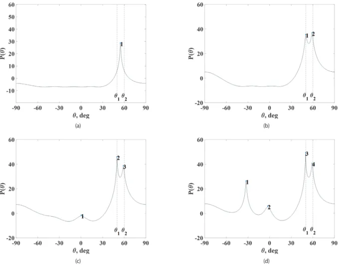
Fig. 2 shows the MUSIC spatial spectrum according to the noise eigenvector's dimensions when the 5-elements ULA receives two signals. The incident angles are 50 deg (θ

) and 60 deg (θ

). Fig. 2a is the spatial spectrum of the 1-dimensional noise eigenvector that has only one peak between θ

and θ

. The 3-dimensional noise eigenvector graph (Fig. 2b) is the correct spatial spectrum, and it has the correct peaks. Figs. 2c and d show incorrect peaks as well as the correct peaks. Note that the incorrect peak's angles are not constant, unlike the correct peaks. If the spectrums are calculated repeatedly using data that is input continuously, the correct peaks continue to appear at similar angles.

On the other hand, the angles of the false peaks change continuously.

Fig. 3 shows the result of the 30 times simulation under the same conditions as in Fig. 2. The bin width of the histogram is 5 deg. It should be determined in consideration of the system resolution performance. It can be seen that the count value of the bin where the input signal exists is higher than the count value of the other bins. Therefore, the NOS can be obtained through the number of bins whose count value is higher than the threshold. The threshold should be determined empirically in consideration of the number of the spatial spectrum calculations.

3.1.2 Detection of false peaks

The system using an array antenna can measure the

DOA using the phase difference of the signals received at

the array elements. The performance of the system related to the geometry of the array elements. Generally, the wider the inter-element spacing, the better the DOA estimation resolution of the system. However, if the inter-element spacing exceeds a certain range, the phase difference will produce ambiguity, which will cause false peak in the

spatial spectrum.

Fig. 4 depicts the simulated spatial spectrums according to the inter-element spacing. In this simulation, 5-elements ULA receives two signals at -20 and +30 deg. The SNRs are the same at 0 dB, and the number of sample data is 200 for each spatial spectrum. In this figure, the red line has a Fig. 2. The spatial spectrum according to the dimensions of the noise eigenvector: (a) 4-D; (b) 3-D; (c) 2-D; (d) 1-D.

(a)

(c)

(b)

(d)

Fig. 3. The histogram graph of the peak values. Fig. 4. The spatial spectrum according to the spacing of the array element.

sharper beam than the black line. It means that the red line has a better resolution performance than the black line.

The blue line is the spatial spectrum when the length of the inter-element spacing is longer than the half-wavelength under the other conditions are the same. It has not only true

peaks but also false peaks. The false peaks on the spatial spectrum have no difference from the true peaks, which makes it difficult to estimate the DOA.

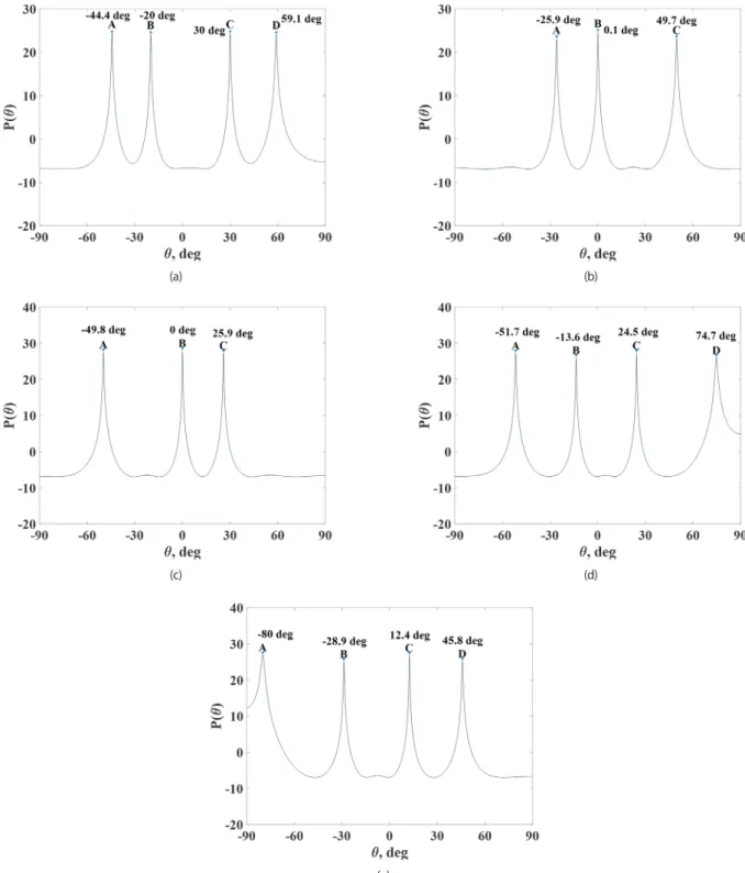
Fig. 5 shows the spatial spectrum simulation when the antenna direction is 0 deg, the true peak directions, and Fig. 5. The spatial spectrum according to the directions of the array antenna: (a) 0 deg direction; (b) -20 deg direction (True peak direction); (c) 30 deg direction (True peak direction); (d) -44.4 deg direction (False peak direction); (e) 59.1 deg direction (False peak direction).

(a)

(c)

(e)

(b)

(d)

the false peak directions. Note that the true peak's angle moves as much as the antenna direction rotates, but the false peak's angle does not. Thus, it is possible to determine whether the peak is false or not by using the peak angle change after rotating the antenna direction. If the peak appears around 0 deg after rotating the antenna direction to the peak, it is a true peak.

3.2 DOA Estimation Method

The proposed DOA estimation method is shown below.

1. Calculate the spatial spectrums using the MUSIC algorithm for whole-dimensional noise eigenvectors at the initial array direction.

2. Find and collect the peak angles on the spatial spectrum.

3. Repeat 1 ~ 2 N

times.

4. Create the histogram for the collected peak values.

5. Find the top 4 bins whose count value exceeds N

. 6. Calculate the average values of the samples included

in each bin.

1 2 3 4

_ _ _ _

avg bin avg bin avg bin avg bin

θ θ θ θ

 

  (12)

7. Rotate the antenna direction to θ

.

8. Calculate the spatial spectrums using the MUSIC algorithm for whole-dimensional noise eigenvectors.

9. Find and collect the peak angles on the spatial spectrum.

10. Repeat 8 ~ 9 N

times.

11. Create the histogram for the collected peak values.

12. Find the top 4 bins whose count value exceeds N

. 13. Calculate the average values of the samples included

in each bin.

14. Find the value closest to 0 deg (θ

).

15. Compare θ

and θ

to see whether it is a true peak or false peak and save the raw data if it is a true peak,

is a true peak, if is a false peak, if

Fine Fine th

Fine th

θ θ

θ θ θ

 ≤ 

 > 

  (13)

16. Repeat 7 ~ 15 for θ

~ θ

.

17. Determine the number of the true peaks. It is the NOS (P).

18. Recalculate the spatial spectrum using the measured NOS and the raw data acquired when the antenna direction is a true peak in 15.

19. Find and collect the peak value closest to 0 deg.

20. Calculate the average of the peak angles obtained at

19 (θ̇

(p), (p = 1, 2, … P)).

21. Determine final DOA value by considering the antenna direction,

( )

Final Fine

p

θ = θ  + θ (14)

The system parameters (N

, N

, N

, θ

, and the bin width of the histogram) are not theoretically derived values, but empirically obtained values. If N

and N

are too small, the system will underestimate the NOS. On the other hand, if these values are too large, the processing time will increase. The value of Nth should be set in proportion to the values of N

and N

. The value of θ

also influences NOS measurement. The system with a small value of θ

underestimates the NOS, and the system with a large value of θ

overestimates the NOS. The histogram bin width should be determined according to the system resolution.

If the bin width is too narrow, the bin count value corresponding to the true peak will not be sufficient. On the other hand, if it is too wide, the system will not be able to distinguish between nearby signal sources.

4. CALIBRATION

The DOA estimation system using the array antenna has multiple channels, and each channel has a different phase delay and gain. These differences cause an error in the DOA estimation, so it is essential to calibrate the system. As the radio wave signal passes through the system hardware, the phase and amplitude are changed. In particular, in the case of an antenna, since the phase delay and amplitude variation depend on the signal incident angle, it is necessary to calibrate the system according to the incident angle. The system calibration proceeds in the following order:

1. Transmit the signal from the known direction,

2. Measure and save the output signal of the receiver according to the direction,

3. Calculate the difference of the phase delay and gain between the reference channel and the target channel, 4. Calculate the correction values for the target channels.

5. Apply the correction values to the system.

The calibration of the DOA estimation system should

be performed in an environment in which unknown error

factors are minimized. The anechoic chamber is a suitable

environment for the calibration because it blocks external

propagation and minimizes multipath. In the anechoic

chamber, the distance between the radio wave source and

the array antenna is several meters. However, the developed system has to measure the signal's DOA that is several kilometers away. Therefore, when calibrating the system, the characteristics of the radio wave must be considered.

First of all, the calibration should be performed under far-field conditions because the developed system operates in the far-field. The condition of far-field is

2 D

l ^≥ λ ⁽¹⁵⁾

where l is the transmission distance, D is the largest dimension of the antenna, and λ is the wavelength of the signal (Balanis 2016).

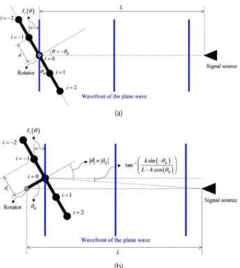
Assuming that the 5-element ULA receives a continuous- wave signal as depicted in Fig. 6, then the output signal of the i-channel can be defined as

( ) ( ) ( )

( ) ( )

( 2, 1, ,2 )

i

H D

i i

j

i i

j j

H D

i i

y t G x t e

G G x t e e i

ωτ θ

ωτ θ ωτ

θ θ

−

− −

= ⋅ ⋅

= ⋅ ⋅ ⋅ ⋅ = − −  (16)

where x(t) is the transmit signal, y

(t) the output signal of the i-channel, θ is the incident angle, G

(θ) is the total amplitude variation from the transmit antenna to the output of the i-channel, G

(θ) is the gain of the i-channel, G

is the propagation loss between the transmit antenna and the array element of the i-channel, e

is the total phase delay from the transmit antenna to the output of the i-channel, e

is the phase delay of the i-channel, e

is the propagation phase delay between the transmit antenna and the array element of the i-channel, and i is the index of the channel. The purpose of the calibration is to equalize the gain and phase delay of all channels.

The gain of the reference channel can be defined as

( ) ( ) ( )

0H H

i i

G θ = G � θ ⋅ G θ (17)

where G

(θ) is the gain of the reference channel and Ĝ

(θ) is the gain correction of the i-channel, and the gain correction can be expressed as

( ) ( ) ( )

( ) ( ) ( )

( ) ( )

( ) ( )

0

0 0 0 0

, 0

H D

D D

i H i

i i i i

D i

G

G G G A

G� G G

G

G G A

G θ

θ θ θ

θ ⁼ θ ⁼ θ ⁼ θ ⁼ θ ^{ ≈}

(18)

where G

(θ) is the total amplitude variation from the transmit antenna to the output of the reference channel, G

is the propagation loss between the transmit antenna and the array element of the reference channel, A

(θ) is the amplitude of the reference channel's output signal, and A

(θ) is the amplitude of the i-channel's output signal. Therefore, the gain correction for the i-channel is determined by the output signal amplitude ratio of the reference channel to the i-channel.

The phase delay of the reference channel can be defined as

( ) ( ) ( )

0^H ˆi i^H

j j j

e

= e

⋅ e

(19)

where e

is the phase delay of the reference channel and e

is the phase correction of the i-channel. If the inter-element spacing is shorter than the input signal's wavelength, then the phase correction can be expressed as

( ) ( )

( ) ( )

( ) ( )

( )

{ ( ) ( ) } ( )

0

0 0 0

0 ˆ

0

H D iD

i

H i i D

i

iD j

j j j j

j

i i

j j

j j

j

e ee e e

e e e e e

e

ωτ θ

ωτ θ ωτ ωτ θ ωτ

ωτ θ

ωτ θ ωτ θ

ωτ θ ωτ

ωτ

φ θ φ θ φ θ

−

− − − −

−

− −

− −

−

= = = ⋅ = − − 

(20)

( )

i

e

φ θ  =

(21)

where e

is the total phase delay from transmit antenna to the output of the reference channel and e

is the propagation phase delay between the transmit antenna and the array element of the reference channel, ϕ

(θ) is the phase of the reference channel's output signal, and ϕ

(θ) is the phase of the i-channel's output signal, and ϕ̃

(θ) and τ̃

(θ) means the propagation phase and time delay difference between the reference channel and the i-channel. Therefore, in order to calculate the phase correction for the i-channel, the propagation time delay difference between the reference channel and the i-channel should be considered as well as the output signal phase difference. Figs. 7 and 8 express the propagation time delay difference according to the test configuration and radio wave characteristic.

In general, the radio wave propagates outward in all directions from its source. If the medium around the source is the same everywhere, the radio wave is transmitted uniformly in all directions. Therefore, the wavefront with the same phase is spherical. It is called a spherical wave.

However, far from the source, the wavefront looks like a

Fig. 6. The block diagram of the calibration.

plane, and it is called a plane wave. If the signal impinges on the array in the form of the plane wave as shown in Fig. 7, the propagation time delay difference can be defined as

( ) ^sin

i

id

c

τ θ  = θ (22)

where d is the inter-element spacing, and θ is the incident angle of the signal.

The rotator can be used to control the incident angle of the signal, as shown in Fig. 7a. In this figure, the rotator is aligned with the transmit antenna. The relation between the incident angle of the signal and the rotator direction angle is

( )

, 90 90

R R

θ = − θ − ≤ θ ≤ (23)

where θ

is the direction of the rotator. If there is a lever-arm as shown in Fig. 7b, the relation is redefined as

( )

( ) ( )

1

sin

tan , 90 90

cos

R R

R

k L k

θ θ θ θ

θ

−

 − 

= − +    −    − ≤ ≤ (24)

where k the lever arm's length and L is the distance between the rotator and the transmit antenna.

Fig. 8 shows the propagation time delay difference of the plane and spherical wave. In this figure, the blue line is the plane wave, and the red line is the spherical wave. The propagation time delay difference for plane and spherical

wave is

( ) ^sin (

)

i

id c

τ θ  = ⁻ θ (for plane wave) (25)

( )

i

c

τ θ  = α β ⁻ (for spherical wave) (26)

( ) ( ( ) )

( ) ( ( ) )

( )

2 2

2 2

, ,

2 2 , 1

cos sin

ˆˆ cos ˆˆ sin ˆ

ˆ tan

R R

i i R i i R i

i

R i R

k L k

k L k

k k id id

k

α θ θ

β θ θ

θ θ

 = − + − 

 

 

 = − + − 

 

 

= +

 

   

 = +   

   

 

(27)

In Eqs. (26) and (27), α is the distance between the transmit antenna and the array element of the reference channel, and β

is the distance between the transmit antenna and the array element of the i-channel. The environment of the anechoic chamber is too close to assuming that the wavefront is planar. Therefore, the propagation phase delay difference should be calculated by considering that the signal is a spherical wave. Fig. 9 shows the difference between the spherical wave's τ̃

(θ) and the plane wave's Fig. 7. The relation between the signal incident angle and the rotator

direction angle: (a) No lever arm; (b) Lever arm's length is k.

(a)

(b)

Fig. 8. The propagation time delay difference of the spherical wave.

Fig. 9. The difference between the spherical wave's τ̃

(θ) and

the plane wave's τ ̃

(θ).

τ̃

(θ). In this figure, the frequency of the signal is 1.6 GHz, i

= 2, d = 13 cm, L = 5 m, and k = 50 cm. It can be seen that the difference is over 30 degrees.

After the phase and gain correction values are calculated according to the incident angles and channels, the correction values are applied to the steering vector, a(θ), in Eq. (11). The system should calculate the spatial spectrum using the calibrated steering vectors.

The steering vector before and after calibration is ( )

aθ = e^−ωτ−θ e^{−ωτ θ−} e^{−ωτ θ} e^{−ωτ θ} (before calibration)

(28)

( )

( )

( )

( )

( )

2 2

1 1

1 1

2 2

2 ˆ 1 ˆ

1 ˆ 2 ˆ

1

j j

j j

j j

j j

G e e

G e e

a

G e e

G e e

ωτ θ ωτ θ

ωτ θ ωτ θ

ωτ θ ωτ θ

ωτ θ ωτ θ

θ θ θ

θ θ

− −

− −

− −

−

− −

−

− −

− −

 ⋅ ⋅ 

 

 ⋅ ⋅ 

 

=  

 ⋅ ⋅ 

 

 ⋅ ⋅ 

 

� � � �

(after calibration) (29)

( ) ^sin ( ) ( 2, 1, ,2 )

i

id i

c

τ θ = θ = − −  (30)

5. FIELD TEST

Fig. 10 shows the developed DOA estimation system.

It consists of 5-element ULA, rotator, receiver, control device, storage device, and other environmental devices.

The spacing of the antenna element is 13 cm, which is longer than the half-wavelength of the GPS L1 signal (about 9.5 cm). The rotator can adjust the azimuth of the array antenna from -90 deg to +90 deg. The forward direction of the antenna is 0 deg, and (+) means the right direction from the forward direction. Table 1 shows the system parameters.

The radio wave signal received by the array antenna is converted into a digital signal at the receiver. The control device estimates the DOA using the digitally converted signal and adjusts the array antenna's direction.

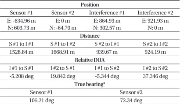
For the test, two interference sources and two DOA estimation systems were installed outdoors in a range of 1.5 x 1.0 km. The test layout is presented in Fig. 11. Table 2 shows the position and distance between the interference sources and the systems and the true bearing of the array antenna.

The true bearing of the array antenna is calculated using the GNSS precise point positioning (PPP) receiver and the digital projector equipped with ripple scope. Fig. 12 shows the picture of the digital projector and the receiver. The true bearing measurement procedure is as follows.:

Fig. 11. The layout of the field test.

Fig. 10. The developed AOA estimation system.

Table 1. The system parameters.

N1 N2 Nth θth Bin width

30 30 10 8 deg 5 deg

Table 2. The test configuration parameters.

Position

Sensor #1 Sensor #2 Interference #1 Interference #2 E: -634.96 m

N: 603.73 m E: 0 m

N: -64.70 m E: 864.93 m

N: 302.57 m E: 921.93 m N: 0 m

S #1 to I #1 S #1 to I #2 S #2 to I #1 S #2 to I #2

1528.84 m 1668.91 m 939.67 m 924.19 m

Relative DOA

I #1 to S #1 I #2 to S #1 I #1 to S #2 I #2 to S #2 -5.208 deg 19.842 deg -5.344 deg 37.346 deg

True bearing*

Sensor #1 Sensor #2

106.21 deg 72.34 deg

*(+) means the right direction based on the true north.

(a) (b)

Fig. 12. (a) Digital projector equipped with ripple scope, (b) GNSS PPP

receiver.

1. Measure the positions of the interferences #1 and the system's array antennas using the PPP receiver.

2. Calculate the angle between the line from the array antenna to the interference #1 (θ

). and the line from the array antenna to the true north.

3. Measure the angle between the front line of the array antenna and the line from the array antenna to the interference #1 using the digital projector (θ

).

4. Calculate the true bearing of the array antenna (θ

),

1 2

θ

= − θ θ (31)

Table 3 describes the example of the step-by-step test results for two 1.585 GHz additive white Gaussian noise (AWGN) signals. The signal's half wavelength is about 9.5 cm, which is shorter than the inter-element spacing (13 cm). In steps 1 to 6, the count value corresponding to 5.32 deg was less than N

, so it was ignored in the next step. The count value corresponding to -56.99 deg was above N

, but the system detected it as a false peak. In steps 15 to 18, the system estimated the DOA values as -5.29 deg and 37.25 deg. The results show that even though the inter-element spacing exceeds the half-wavelength of the input signals, the system correctly detects the false peak and determines

the NOS by the proposed algorithm.

The L-band interference DOA estimation tests were performed to evaluate the performance of the system. Table 4 presents the test scenarios, and the system estimates the DOA three times for each scenario. The frequency and power level of the interferences are determined in consideration of the test range condition. In Figs. 13 and 14 show the average DOA estimation error for each scenario.

As a result of measuring a single interference, the system

#1 showed a result that was biased toward the '-' direction and system 2 showed a result that was biased toward the '+' direction. This error is due to the position error that occurs when the GNSS receiver measures the position of the system and the direction error that occurs when the digital projector measures the direction of the system. However, it is difficult to observe this bias in the test results for dual jammers, because multiple signals present at the same frequency distort the spatial spectrum. The measurement performance of a DOA measurement system using an array antenna improves as the angle of incidence decreases, but such a trend is not observed in this test. The reason is that the system developed in this paper measures the DOA of Table 3. System #2’s step-by-step test results for AWGN interferences.

Step Ant.

Dir.**

(deg)

#1 #2 #3 #4 True

or False DOA*

(deg) Count DOA

(deg) Count DOA

(deg) CountDOA (deg)Count

1 ~ 6 0 -56.99 25 38.5 24 -5.87 15 5.32 5 -

7 ~ 14 -56.99

-5.87 27.19 -50.24 15

22 -44.18 43.86 13

22 49.42 1.27 13

20 -

- -

- FALSE TRUE

- 5.32 Ignored (The count value is less than N

) TRUE

38.5 0.02 30 49.74 18 -43.71 14 - -

15 ~ 18 - -5.29 - 37.25 - - - - - -

*DOA is a relative value for the antenna direction.

**The antenna direction is a relative value for the true bearing.

Table 4. The L-band interference DOA estimation test scenarios.

Test #

Single

Test #

Dual Freq

(MHz) SNR (dB) BW

(MHz) Freq

(MHz) SNR (dB) BW

(MHz) Freq (MHz) SNR

(dB) BW (MHz)

1

2 3 4 5 6 7 8

1235 1235 1250 1220 1585 1585 1600 1570

20 20 20 20 20 20 20 20

0*

5 20 20 0*

5 20 20

1 2 3 4 5 6 7 8 9 10

1235 1235 1235 1235 1220 1585 1585 1585 1585 1570

20 2 20 0*

0*

2 2 20 0*

0*

2 1235 1235 1250 1220 1250 1585 1585 1600 1570 1600

25 2 20 2 20 20 2 20 2 20 20

* 0 MHz mean a single-tone signal.

Fig. 13. The single L-band interference DOA estimation test results.

Fig. 14. The dual L-band interference DOA estimation test results.

the signal from the front through the direction control of the antenna. The estimation accuracy was 0.56 deg (RMS) for single interference and 0.9 deg (RMS) for dual interference.

6. CONCLUSIONS

This paper describes the development and field test results of the 5-element ULA DOA estimation system.

In order to measure the NOS, the system utilizes the characteristic of the peak occurrence frequency according to the noise eigenvector's dimension. Also, the system detects the false peaks by using the false peak's angle variation characteristic according to the antenna's direction moving. To calibrate the system, we consider the anechoic chamber environment and the radio wave propagation characteristics. The results of the field test show the validity of the developed system.

The proposed algorithm effectively measured the NOS and detected the false peaks, but it takes time in the process of iteratively calculating the spatial spectrum and mechanically controlling the antenna direction. This makes the developed system difficult to apply in real time.

Therefore, in order to improve the algorithm, it is necessary to reduce the number of the spatial spectrum calculations and to control the antenna direction electronically.

The system will be deployed on the site and applied to the L-band interference geolocation system.

AUTHOR CONTRIBUTIONS

Conceptualization, S. Seo and K. Song; methodology, S.

Seo, Y. Park, and K. Song; validation, S. Seo; writing-original draft preparation, S. Seo; writing-review and editing, Y.

Park, and K. Song.

CONFLICTS OF INTEREST

The authors declare no conflict of interest.

REFERENCES

Akbari, F., Moghaddam, S. S., & Vakili, V. T. 2010, MUSIC and MVDR DOA Estimation Algorithms with Higher Resolution and Accuracy, in 5th International Symposium on Telecommunications, Tehran, Iran, 4-6 Dec 2010. https://doi.org/10.1109/ISTEL.2010.5734002

Balaei, A. T., Motella, B., & Dempster, A. G. 2007, GPS Interference Detected in Sydney-Australia, in International Global Navigation Satellite Systems Society Symposium, Sydney, Australia, 4-6 Dec 2007 Balanis, C. A. 2016, Antenna Theory: Analysis and Design

4th ed. (New Jersey: John Wiley & Sons), pp.31-33 Chen, W., Wong, K. M., & Reilly, J. P. 1991, Detection of

the Number of Signals: A Predicted Eigen-threshold Approach, IEEE Transactions on Signal Processing, 39, 1088-1098. https://doi.org/10.1109/78.80959

Dempster, A. G. & Cetin, E. 2016, Interference Localization for Satellite Navigation Systems, Proceedings of the IEEE, 104, 1318–1326. https://doi.org/10.1109/

JPROC.2016.2530814

Di, A. & Tian, L. 1984, Matrix Decomposition and Multiple Source Location, in ICASSP '84. IEEE International Conference on Acoustics, Speech, and Signal Processing, San Diego, CA, USA, 19-21 Mar 1984.

https://doi.org/10.1109/ICASSP.1984.1172651

Evans, S. 2016, British Broadcasting Corporation, North Korea 'jamming GPS signals' near South border, British Broadcasting Corporation. Retrieved from https://

www.bbc.com/

Jiang, J. S. & Ingram, M. A. 2004, Robust Detection of Number of Sources Using the Transformed Rotational Matrix, in 2004 IEEE Wireless Communications and Networking Conference, Atlanta, GA, USA, 21-25 Mar 2004. https://doi.org/10.1109/WCNC.2004.1311595 Manikas, A. & Proukakis, C. 1998, Modeling and Estimation

of Ambiguities in Linear Arrays, IEEE Transactions on Signal Processing, 46, 2166-2179. https://doi.

org/10.1109/78.705428

Motella, B., Pini, M., & Dovis, F. 2008, Investigation on the Effect of Strong Out-of-Band Signals on Global Navigation Satellite Systems Receivers, GPS Solutions, 12, 77-86. https://doi.org/10.1007/s10291-007-0085-5 Pullen, S., Gao, G., Tedeschi, C., & Warburton, J. 2012, The

Impact of Uninformed RF Interference on GBAS and Potential Mitigations, in 2012 International Technical Meeting of the Institute of Navigation, Newport Beach, CA, USA, 30-31 Jan 2012

Reed, S., Mallett, J. D., & Brennan, L. E. 2004, Rapid C o n v e r g e n c e R a t e i n A d a p t i v e A r r a y s, I E E E Transactions on Aerospace and Electronic Systems, 10, 853-863. https://doi.org/10.1109/TAES.1974.307893 Schmidt, R. 1986, Multiple Emitter Location and Signal

Parameter Estimation, IEEE Transaction on Antennas and Propagation, 34, 276-280. https://doi.org/10.1109/

TAP.1986.1143830

Wax, M. & Kailath, T. 1985, Detection of Signals by

Information Theoretic Criteria, IEEE Transactions on Acoustic, Speech, and Signal Processing, 33, 387-392.

https://doi.org/10.1109/TASSP.1985.1164557

Yuri, N. & Ilia, P. 2016, Probability of False Peaks Occurring via Circular and Concentric Antenna Arrays DOA Estimation, in 2016 39th International Conference on Telecommunications and Signal Processing, Vienna, Austria, 27-29 Jun 2016. https://doi.org/10.1109/

TSP.2016.7760854

Seungwoo Seo is a senior researcher of Agency for Defense Development in Korea, Republic of. He received B.S. and M.S degree in electrical engineering at Korea University.

His research interests include time synchronization system and array signal processing.

Youngbum Park received the Doctor’s degree in Aerospace engineering from Seoul National University in 2017. Since 2001, he has been working for Agency for defense development. His research interests include estimation, localization, and integrated navigation system.

Kiwon Song received the Doctor’s degree in

Electronics engineering from Chung-nam

National University in 2002. His research

interests include design of satellite

navigation system architecture, GNSS signal

generation processing, and integration

optimal filter of INS/GPS.