Non-hydrostatic modeling of nonlinear waves in a circular channel

제 23 권 제 5 호, pp. 335~344, 2011년 10월

335

Non-hydrostatic modeling of nonlinear waves in a circular channel 비정수압 모형을 이용한 원형 수로에서 비선형 파랑의 해석

Doo Yong Choi*

최두용*

Abstract : A curvilinear non-hydrostatic free surface model is developed to investigate nonlinear wave interactions in a circular channel. The proposed model solves the unsteady Navier-Stokes equations in a three-dimensional domain with a pressure correction method, which is one of fractional step methods. A hybrid staggered-grid layout in the vertical direction is implemented, which renders relatively simple resulting pressure equation as well as free surface closure. Numerical accuracy with respect to wave nonlinearity is tested against the fifth-order Stokes solution in a two-dimensional numerical wave tank. Numerical applications center on the evolution of nonlinear waves including diffraction and reflection affected by the curvature of side wall in a circular channel comparing with linear waves. Except for a highly nonlinear bichrmatic wave, the model’s results are in good agreement with superimposed analytical solution that neglects nonlinear effects. Through the numerical simulation of the highly nonlinear bichramatic wave, the model shows its capability to investigate the evolution of nonlinear wave groups in a circular channel.

Keywords : non-hydrostatic model, curvilinear coordinate, nonlinear wave, wave diffraction, wave reflection

요 지 : 곡면의 경계를 가지는 수로에서 비선형 파랑의 상호작용을 모의하기 위한 비정수압 자유수면 모형이 개

발되었다. 제안된 모형은 비선형의 3차원 Navier-Stokes 방정식을 곡선좌표 영역에서 계산단계 분리법의 일종인 압 력수정법에 의하여 수치적으로 해석된다. 특히, 연직방향으로 변형된 형태의 엇갈린 격자를 이용하여 상대적으로 간 단하게 압력방정식과 자유수면 경계조건을 구성하였다. 개발된 모형의 수치해석 정확도는 2차원의 수치 파수조에서 파랑의 비선형 정도에 대하여 5차의 스토스우크스 해석해와 비교하였다. 본 모형의 실제적 적용은 원형의 수로에 서 회절과 반사에 의해 변형되는 비선형 파의 변형에 초점을 맞추어 수행하였다. 두개의 파를 중첩한 고비선형의 파에 대한 경우를 제외하고 수치해석 결과는 비선형적인 영향을 고려하지 않은 해석해의 선형적인 중첩과 일치하 였다. 두개의 파를 중첩한 고비선형의 파에 대한 모의를 통하여 본 모형은 원형의 수로에서 비선형 군파의 변형에 관한 수치적인 모의 가능성을 제시하였다.

핵심용어 : 비정수압 모형, 곡선좌표, 비선형 파랑, 파의 회절, 파의 반사

1. Introduction

The understanding of wave propagation through curved channels is essential in engineering applications that involve winding turns in rivers, harbors, and canals. Earlier theoretical research found that the propagation of linear waves was influenced by the sharpness of the channel bend (Rostafinski, 1972; Rostafinski, 1976). Subsequent numerical modeling revealed that both wave reflection and diffraction play an important role in the evolution of short waves, and that the reflection of short waves was so strong that the growth of a Mach stem at the outer wall of a channel bend was observed (Kirby, 1988; Kirby et al., 1994).

To date, only a few numerical models have been successfully used to elucidate the evolution of waves in curved channels due to the extensive computational resources that are required.

This challenge has mainly been addressed using depthintegrated wave models: the parabolic equation (Kirby, 1988; Kirby et al., 1994; Shi and Kirby, 2005; Zhang et al., 2005), a Boussinesq-type equation (Shi et al., 1998; Li and Zhan, 2001), and a hyperbolic equation (Beji and Nadaoka, 2004). The application of these models, however, was accomplished in weakly and intermediately dispersive waves (e.g., at a dimensionless relative water depth of Kh ~2.5, where K and h are the wave number and water depth, respectively), until highly dispersive waves (e.g., Kh =π) were later

*한국수자원공사 K-water연구원 (K-water Research Institute, Korea Water Resources Corporation, 462-1 Junmin-dong, Yuseong-gu, Daejeon 305- 370, Republic of Korea. Tel.:+82 42 629 3837; fax: +82 42 629 3839; e-mail address: [email protected])

*

explored using a three-dimensional (3D) non-hydrostatic model developed by the author (Choi et al., 2011). This may be attributable to the fact that only limited efforts were made to alleviate the constraints of depthintegrated models, which include weak nonlinearity and frequency dispersion in the curvilinear domain. Choi et al. (2011) showed that the complexity of the resulting waves increased depending on the degree of dispersion. Nonetheless, the numerical application of the previous paper was not explored due to the unavailability of an analytical solution, as well as numerical restrictions, which will be described below.

In recent decades, many non-hydrostatic models have been developed to effectively capture the moving airwater interface by solving the related incompressible Navier-Stokes equations (NSEs) (Mahadevan et al., 1996; Casulli, 1999; Li and Fleming, 2001; Armfield and Street, 2002; Lin and Li, 2002;

Stelling and Zijlema, 2003; Yuan and Wu, 2004; Bradford, 2005; Young et al., 2009; Choi et al., 2011). In these models, the free surface elevation is defined as a single-valued function of horizontal positions from the kinematic free surface equation.

Unlike other approaches, such as the marker-and-cell (MAC) method (Harlow and Welch, 1965) and the volume-of-fluid (VOF) method (Hirt and Nichols, 1981), these non-hydrostatic models track free surface wave motions with relatively small computational expense. Moreover, the most remarkable development in non-hydrostatic modeling is the employment of a small number of vertical layers (i.e., two to five layers); this approach is comparable to the depth-integrated type model in terms of computational efficiency (Stelling and Zijlema, 2003;

Yuan and Wu, 2004; Young et al., 2009; Choi et al., 2011).

These approaches, however, still have an overshooting issue in the modeling of nonlinear waves in which the wave trough is below the bottom of the top vertical layers in the Cartesian coordinate system. The introduction of a σ-coordinate system in the vertical direction may alleviate this overshooting issue by ideally mapping the propagation of nonlinear waves, but it requires more computational layers (i.e., computational diagonals in the pressure Poisson equation) due to the crossdifferential terms of σ-transformation, particularly in the fractional step method.

In this paper, we adopt a hybrid staggered-grid arrangement, which was originally proposed by Ai et al. (2010), in order to effectively resolve the crossdifferential terms in the σ- coordinate system. Meanwhile, the pressure correction method of Kang and Fringer (2005) is implemented in the fractional time integration, combined with the second-order Adams- Bashforth scheme and the thirdorder spatial upwind method

for the advection terms in the three-dimensional (3D) curvilinear coordinates. Furthermore, the free surface elevation is updated by discretizing the free surface equation with a forth-order spatial scheme to resolve the steep-surface wave propagation. The numerical accuracy of the developed model is first tested against analytical solutions for a two-dimensional numerical wave tank for nonlinear Stokes waves with different values of wave steepness, i.e., aK = 0.1, 0.2, and 0.3, where a is the wave amplitude. Numerical applications are focused upon 3D nonlinear wave transformation in a curved channel with an intermediate water depth. Because highly refined horizontal grids must be employed in order to capture the dispersion of deepwater waves, as reported in a previous study, numerical attention is only paid to the evolution of nonlinear waves with an intermediate water depth. The first example addresses the nonlinear evolution of monochromatic waves, including the diffraction and reflection produce by the curved sidewall. Next, the model is applied to the simulation of bichromatic waves as influenced by amplitude differences.

2. Mathematical formulation in a curvilinear coordinate

Three-dimensional (3D) free surface flow is governed by incompressible Navier-Stokes equations (NSEs), which represent the conservation of mass and momentum. The primitive variable forms of the governing equation in the Cartesian coordinate are written as

(1)

subject to the continuity constraint

∇ ·u = 0, (2)

where t is the time, ∇² is the Laplacian operator, ∇ is the gradient, and u, e, f, g and p are given by

(2)

where u, v and w are the fluid velocities in the x−, y−, and z− direction, respectively; p is the normalized pressure divided by a constant reference density; is the gravitational acceleration; and vt is the eddy viscosityg coefficient.

In order to model a time-dependent irregular domain, independent variables t, x, y, and z− in the physical space are transformed into τ, ξ, ζ, and σ in the computational space,

∂ u --- ∂∂ t e

∂ x--- ∂f

∂ y--- ∂g

∂ z---

+ + + = –p+vt∇²u

u u

v w

, e uu vu wu

, f uv vv wv

, g uw vw ww

, p ∂ p ∂ x⁄

∂ p ∂ y⁄

∂ p ∂ z g⁄ +

= = = = =

while dependent variables are converted into contravariant variables. In the vertical domain, the σ-coordinate system is used to conform to an undulating bottom topography and the timedependent free surface is defined as

(3)

where H is the total water depth. Note that σ transformation results in σ = −1 at the bottom and σ = 0 at the free surface. In the horizontal space, the computational domain is mapped onto smooth curvilinear grids, expressed as ξ, ζ, that remain fixed in time. By defining the coordinate transformation between the Cartesian and curvilinear spaces as

τ = t, ξ = ξ (x, y), ζ = ζ(x,y), and σ = σ(t,x,y,z), (4) the chain rule for partial differential equations becomes

(5)

where the subscripts of the metrics denote the partial derivatives, e.g., ∂ξ/∂ x = ξx, and JH is the Jacobian of the horizontal transformation, which is defined as |x_ξy_ζ− y_ξx_ζ| =σzJ.

By substituting Eq. (5) into Eqs. (1) and (2), a step that introduces the contravariant velocities that are perpendicular to the ζ, ξ-curvilinear coordinates expressed in terms of the Cartesian velocities as U =ξxu +ξyv, V =ζxu +ζyv, and by defining the sigma velocity as W =σt+σxu +σyv +σyw, the curvilinear form of the governing equations in terms of the transformed variables becomes

(6)

where U, E, F, G, H, and P are given by

,

and is the Laplacian of the Cartesian velocity in the diffusion terms. Similarly, the continuity equation of (2) can be transformed into

(7)

or

(8)

It should be noted in the kinematic boundary conditions that W is zero at the free surface and at the bottom.

Among all the boundary conditions, the Dirichlet-type boundary conditions that give specific values of variables can remain in the same condition as the Cartesian coordinate.

However, the Neumann-type boundary conditions that involve partial differentiation should be transformed into the curvilinear plane. First, the moving boundary condition of the free surface can be written into

(9) In addition, a null gradient condition for the tangential velocity components against the wall⎯the socalled free-slip condition (e.g., ∂ U/∂σ = 0)⎯is applied, assuming an inviscid flow in the wave applications.

3. Numerical methods

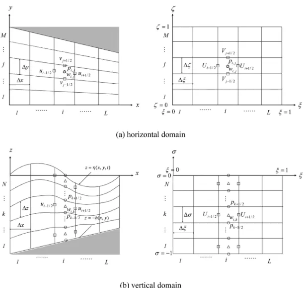
In order to completely impose an atmospheric pressure condition at the free surface, the new grid arrangement of Ai et al. (2010) is applied in the 3D curvilinear coordinate framework, as shown in Fig. 1. An irregular physical domain is mapped into rectangular prisms in the computational space, whose vertical direction is timedependent; they are discretized by L, M and N in the ξ−, ζ−, and σ-directions, respectively.

A deviation from the standard staggered system is made in the variable assignment of vertical velocity w and pressure p. This arrangement of variables eliminates the cumbersome interpolation of nonpositioned vertical velocities while σ z–η

h+η --- z–η

---H ,

= =

∂ ∂t⁄

∂ ∂x⁄

∂ ∂y⁄

∂ ∂z⁄

1 0 0 σt

0ξxζxσx

0ξyζyσy

0 0 0 σz

∂ ∂τ⁄

∂ ∂ξ⁄

∂ ∂ζ⁄

∂ ∂σ ⁄

=

1 0 0 –z_τ⁄z_σ

0 y_ξ⁄JH–y_ξ⁄JH(y_ξz_ζ–y_ζz_ξ) J⁄ H

0 x_ξ⁄JH –x_ξ⁄JH(x_ζz_ξ–x_ξz_ζ) J⁄ H

0 0 0 1 z⁄ _σ

∂ ∂τ⁄

∂ ∂ξ⁄

∂ ∂ζ⁄

∂ ∂σ ⁄

=

∂U--- ∂∂τ E

∂ξ--- ∂F

∂ζ--- ∂G

∂σ--- H

+ + + + = –P+vt∇ξζσ2 u,

U U

V w

, E UU

UV Uw

, F VU

VV Vw

, G UW

VW wW ,

= = = =

H J_H ^1– (y_ζx_ξξ–x_ζy_ξξ)U²+2 y( _ζx_ξζ–x_ζy_ξζ)UV y+( ζx_ζζ–x_ζy_ζζ)V² x_ξy_ξξ–x_ζy_ξξ

( )U²+2 x( _ζy_ξξ–y_ξx_ξζ)UV x+(ξy_ζζ–y_ξx_ζζ)V² 0

,

=

P =

∇ξζσ2

∂ U

∂ ξ--- ∂V

∂ ζ--- σx

∂ U

∂ σ--- σy

∂ V

∂ σ--- σz

∂ w

∂ σ---

+ + + + =0,

∂ U∂ ξ--- ∂V

∂ ζ--- J_H ^1–(y_ξz_ζ+y_ζz_ξ)∂U

∂ σ--- J_H ^1–(x_ζz_ξ+x_ξz_ζ)∂V

∂ σ--- z_σ^–1∂ w

∂ σ---

+ + + + =0

∂ η∂ τ--- 1 JH

--- ∂

∂ ξ---^[∫_–⁰₁(JHHU) σd ^] _J¹

H

--- ∂

∂ ζ---^[∫_–⁰₁(JHHV) σd ^]

+ + = 0

maintaining the staggered grid layout. Furthermore, it prevents the number of diagonals from expanding in the pressure Poisson equation (PPE), particularly in the time- dependent σ-coordinate. The distinctive numerical methods employed are presented in detail in the next section.

3.1. Pressure correction time marching in momentum equations

The pressure correction method follows a fractional step procedure: At each time step, a projected velocity field is first obtained, then the PPE is solved to provide a pressure field by accounting for the divergence-free flow field, and finally, the velocities are updated in the next time step. Unlike the conventional fractional step method (or the projection method), the second-order pressure correction method retains an explicit pressure gradient at the predictor step in order to avoid splitting error (Armfield and Street, 2002).

The second-order time integration of (6) is given by

(10)

By splitting Eq. (10), followed by the fractional step pro- cedure to obtain the predicted velocity field, the advecion-dif- fusion terms, including an approximate pressure field in the momentum equations, are discretized as

(11)

where ∆τ is the time step; superscripts n-1, n, and n+* are the n-1^th, n^th, and intermediate time steps, respectively. In the above formulation, the advection terms are approximated by the second-order Adams-Bashforth scheme in time,

U^{n 1+} –Uⁿ τ ---∆ 1

2--- – 3 ∆E

ξ ---∆ ∆F

ζ ---∆ ∆G

σ ---∆ H

+ + +

⎝ ⎠

⎛ ⎞ⁿ ∆E

ξ ---∆ ∆F

ζ ---∆ ∆G

σ ---∆ H

+ + +

⎝ ⎠

⎛ ⎞^{n 1–}

–

=

P ^{n 1+}

– v_t

---2(∇ξζσ 2 u^{n 1+} +∇ξζσ 2 uⁿ), +

U^{n *+} –U ⁿ τ ---∆ 1

2--- – 3 ∆E

ξ ---∆ ∆F

ζ ---∆ ∆G

σ

∆--- H

+ + +

⎝ ⎠

⎛ ⎞ⁿ ∆E

ξ ---∆ ∆F

ζ ---∆ ∆G

σ ---∆ H

+ + +

⎝ ⎠

⎛ ⎞^{n 1–}

–

=

P ^{n *+}

– v_t

2---(∇ξζσ 2 u^{n *+} +∇ξζσ 2 uⁿ), +

Fig. 1. Coordinate transformation from physical to computational space and variable assignments in a hybrid grid system.

and the viscous terms are approximated by the second- order CrankNicholson scheme. In the spatial domain, either the upwind or the EulerianLagrangian scheme can be used the advection terms, the thirdorder upwind scheme is employed in this study. The diffusion term is discretized using the commonly employed central difference scheme.

In the second step, the predicted intermediate velocities are corrected with the gradient of the pressure correction (Pn+1−Pn) in order to satisfy the divergencefree condition in the continuity equation (7). The momentum equations, Eq. (6), are written in the corrector step, as follows:

(12)

3.2. Spatial discretization of continuity equation Due to the use of hybrid staggered grids in the curvilinear coordinate system, a distinct discretization in space is made from the standard form of equations. In each computational cell, except for the bottom halfcell (i.e., k = 1, 2, …, N-1), the discretized continuity equation (7) at the center of vertical cell face (i, j, k+1/2) is taken to be

(13) Note that because no boundary condition at the bottom is imposed in Eq. (13), further discretization of the continuity equation is essential for the bottom halfcell.

At the bottom, the kinematic boundary condition at the impermeable bottom⎯the velocity normal to the wall is zero⎯can be expressed as Wi, j,1/2= 0 in the curvilinear coordinate. Employing an impermeable condition and assuming the freeslip condition for horizontal velocity components, the continuity equation for the bottom halfcell can be approximated as

(14) where ∆σ1/2=∆σ1/2.

3.3. Pressure correction and free surface update The Poisson equation for pressure correction can be obtained by substituting Eq. (12) into Eqs. (13), and (14), i.e.,

A(Pⁿ⁺¹− Pⁿ) = B (15)

where the coefficient matrix A is sparse, having dimensions of (L × M × N) × (L × M × N), and B is the known vector with (L × M × N). The sparse matrix has 27 diagonals over three layers, which is symmetric and positive definite. Thus, it can be solved by an iterative solver using the preconditioned conjugate gradient method (Casulli, 1999). Once the pressure correction terms are obtained, the corresponding velocity field is updated from Eq. (12). Lastly, the free surface elevation is determined from the discretized form of the free surface equation, which uses the fourthorder spatial scheme to resolve the highly nonlinear wave propagation, as shown below:

(16)

4. Model verification against nonlinearity

To examine the model’s capability for simulating nonlinear waves, a specific deep-water wave case (i.e., Kh =π) was tested using several wave steepness values: aK = 0.1, 0.2, and 0.3. A numerical wave tank (NWT) with a length of 12 incident wavelengths and a still-water depth of 1 m was used as a testing platform. The last two wavelengths served as sponge layers. The fifth-order Stokes theory (Fenton, 1985) was applied in order to impose incident waves at the inflow boundary. A ramp function⎯fr(t) = 1/2[1 + tanh(t− 2T)/T], where T is the wave period⎯was used in order to eliminate spurious oscillations caused by the impulse motion in the initial stage of the simulation. The computational domain was discretized horizontally with 60 grids per wavelength, and vertically with three and five stretching layers, in which the stretching factor of δ = (∆σlower/∆σupper) was 1.33 (Mayer et al., 1998). The time step was determined by setting the Courant number at Cr = (c·∆t)/∆x = 0.5, where c is the wave speed.

The simulated results of the free surface profile were compared with the time differentiation (i.e., ∂ /∂ t) of the velocity potential, φ, which was determined from the fifth-order U ⁿ⁺¹–U^n+*

τ

---∆ =–(Pⁿ⁺¹–Pⁿ)

Stokes solution of Fenton (1985) as follows:

(17)

where clinear is the linear wave celerity, cfifth is the fifth-order wave celerity, and Aij represents the coefficients in the fifth-order solution, depending on the wave number and water depth. The model’s phase and amplitude accuracies over nonlinearity were measured at x = 5L by normalized errors εc= (c_model− cfifth)/c_fifth and εa= (ηmodel− ηfifth)/ηfifth, respectively. In addition, the normalized errors of the linear theory, i.e., εc= (clinear− cfifth)/cfifth and εa= (ηlinear− ηfifth)/ηfifth

were measured for the sake of comparison.

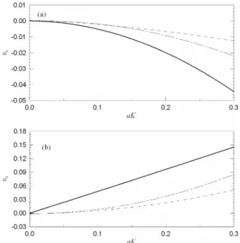
Fig. 2(a) shows the normalized phase error εc over aK.

The relative phase error remained within 1.0% up to aK = 0.2, and increased 2.2% and 1.2% at aK = 0.3 for three and five layers, respectively. The model’s error for resolving the nonlinear phase was less than that of the linear solution, i.e., 4.4% at aK = 0.3. Further describing the nonlinear effect with respect to the normalized amplitude error εa, as shown in Fig. 2(b), the proposed model resulted in 8.5% and 5.0% of normalized errors for aK = 0.3, which was

measured at x = 5L for three and five layers, respectively.

This result indicates that the error of amplitude for a highly nonlinear wave depends on the vertical resolution. Overall, the relative errors regarding phase and amplitude were more accurate than those produced by the linear theory and the other σ based models that require 1020 vertical layers (Li and Fleming, 2001; Lin and Li, 2002). In addition, the main advantage of the present model’s performance can be found in its spatial accuracy, which was produced without significant numerical damping as the nonlinear wave propagated. Fig. 3 shows the predicted spatial distribution of free surface displacement for aK = 0.1, 0.2, and 0.3 at a fully developed stage (t = 30T). In particular, the fivelayer model can accurately predict the free surface profile even for a highly nonlinear wave, i.e., aK = 0.3. In general, the present model reliably predicts vertically asymmetric wave profiles with a higher and narrower crest, as well as a wider and shallower trough as the wave steepness increases.

5. Nonlinearity of monochromatic waves in a circular channel

In their last numerical test, Choi et al. (2011) showed the dispersion effect of linear waves in a circular channel up to a highly dispersive waves (i.e., Kh =π). In this paper, the author aims to investigate the transformation of nonlinear waves in a circular channel by comparing both the linear (i.e., aK = 0.001) and nonlinear (i.e., aK = 0.1) incident waves. The corresponding water depth is chosen to be 1.0 m, in φ x z t( , , ) =

clinear

g K³ ---

⎝ ⎠⎛ ⎞^{1 2⁄} (aK)ⁱ

i=1

∑5 ^Aij j=1

i

∑ ^{cosh( jKz)sin[ jK x c( – fiftht)]}

Fig. 2. Error analysis for wave nonlinearity: (a) phase error over wave steepness, and (b) amplitude error over wave steepness;

linear solution (solid line), three-layer model (dashed-dotted line), and five-layer model (dashed line).

Fig. 3. Comparison of the predicted free surface elevation over space at t = 30T for ak = 0.1, 0.2, and 0.3; analytical solution (solid line), three-layer model (x marks), and five-layer model (circles).

order to be an intermediately dispersive wave (i.e., Kh = 2.11).

The inner and outer walls of the circular channel had radii of 20 and 30 m, respectively. The horizontal domain was discretized into a constant angular grid spacing of π /600 radian, and uniform radial grids of 60, respectively, while additional two wavelengths served as a sponge layer in order to minimize wave reflection from the outgoing boundary. Five vertical layers were employed with a stretching factor of δ = 1.33. The time step was determined by dividing the wave period by 100, and the corresponding Courant number Cr became 0.227.

To obtain the analytical prediction of free surface elevation in a nonlinear wave in a qualitative sense, the author superimposed the linear solution of harmonic waves from the first to the fifth using Fenton’s fifth-order Stokes theory (1985). Note that the superimposed solution has a limitation to be shown as an exact analytical solution because it neglects nonlinear interactions of wave-wall and wave-wave in a circular channel. Mathematically described in a polar coordinate system (r, θ, t), the resulting superimposed solution of the free surface can be written as the summation of the linear combinations of different modes with respect to the Bessel functions of the first and the second kind (Rostafinski, 1976), i.e.,

, (18)

where is the index of harmonic waves, n is the index of modes, Nm is the total number of modes in a single wave m, vn is the order of the Bessel functions, (kr) is the Bessel function of the first kind, (kr) is the Bessel function of the second kind, and an and bn are the amplitudes determined by the solution modes and incident wave conditions. The details of the process of determining the order of the Bessel function can be found in the references (Beji and Nadaoka, 2004; Choi et al., 2011).

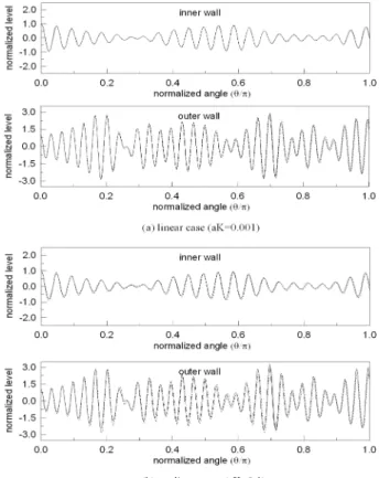
Figs. 4 shows a spatial comparison of the free surface profiles obtained by numerical simulation and by superimposed analytical solutions at the inner wall and outer wall for two different wave steepnesses. The numerical results are in good agreement with the superimposed analytical solutions of five harmonic waves. By comparing Figs. 4(a) and 4(b), it was also found that the wave nonlinearity as expressed by steepness was not a prevailing factor for the spatial distribution of wave height from a normalized point of view. Therefore, wave dispersion driven by the curvature effects of reflection and diffraction would be the most significant factor in the

modulation of monochromatic waves in a relatively deep water condition. This feature is consistent with the qualitative results for an asymmetric Stokes wave reported by Beji and Nadaoka (2004), which demonstrates that the sharp peaks of a Stokes wave are not as prominent as those of a shallow cnoidal wave.

6. Nonlinearity of bichromatic waves in a circular channel

The model was further applied to examine the effects of amplitude differences on nonlinear wave-wave interactions.

Two different waves were chosen for investigation in terms of wave amplitude: one for the case of a small amplitude of 0.02 m (i.e., a weakly nonlinear case), and the other for a larger amplitude of 0.04 m (i.e., a highly nonlinear case).

All computational conditions were set based on high- frequency waves, using the same wave period of 1.4 s as was used in the previous monochromatic example. The bichromatic waves were generated by superimposing high-frequency upon lowfrequency waves that have a wave period of 2.0 s, so the corresponding Kh becomes 1.20.

η r θ t( , ,) [a_nJ_vn( ) bkr + nY_vn( )kr]e^{1 v(nθ ωt+ )}

n 1= N_m m 1= ∑

∑5

=

Jv_n

Yv_n

Fig. 4. Comparison of spatial wave profiles along inner wall and outer wall for (a) a linear case, and (b) a nonlinear case:

superimposed analytical solutions (dotted line), and numer- ical results (solid line).

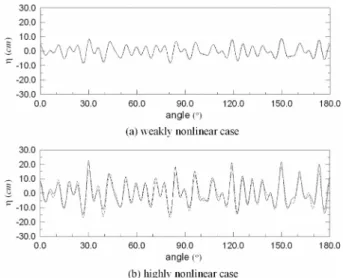
Fig. 5 shows the spatial distribution of wave profiles at one of the fully developed stages, i.e., t = 80Thigh, where Thigh is the wave period of a high frequency wave, in the outer wall. In a comparison of the similarities and differences between the numerical results and superimposed analytical solutions, two interesting points can be addressed here. First, the overall wave profiles are similar for all cases, independent of wave amplitudes. This indicates that the wave dispersion caused by a curved boundary is still dominant in the propagation of bichromatic waves. Second, the differences in amplitude of the numerical and superimposed analytical solutions can be observed in the crests and troughs of a highly nonlinear wave. As shown in Fig. 5(a), the numerical results in the weakly nonlinear case accurately matching the superimposed solutions, which explains the effectiveness of the linear superimposition of analytical solutions. In contrast, the numerical results for a highly nonlinear wave begins with different wave amplitude from 0 degrees because of the combined effect of the nonlinear wave components (see Fig. 5(b)). As the wave trains travel over a channel, the envelope of the numerical results predicts higher crests and lower troughs than does the superimposed solution. This can be explained by the effects of nonlinear wave interactions with the other scattering waves generated by the curved dispersion effect. To better understand the energy transfer involved, a spectral analysis using the fast Fourier transformation (FFT) was carried out for the fully developed waves, which were plotted with regard to the amplitude spectra, as shown in Fig. 6. The amplitude spectrum in Fig. 6(b) shows that the high-frequency wave component interferes more with

the other scattering waves than does the low-frequency component. From the results of the numerical experiments, it may be concluded that more significant nonlinear effects are found for highly nonlinear waves. Fig. 7 shows perspective views of the fully developed wave field.

7. Summary and conclusions

In this paper, a curvilinear non-hydrostatic free surface model was developed in a vertically hybrid staggered grid system.

The model’s accuracy with respect to nonlinear Stokes waves showed satisfactory results as compared to analytical solutions in 2D NWT for different wave steepnesses, i.e., aK = 0.1, 0.2, and 0.3. The proposed non-hydrostatic free surface model was applied to the simulation of waves in a curved channel, with a focus on the nonlinear evolution of Stokes waves in an intermediate water depth. The model results were compared with the superimposed linear solution of harmonic waves, which may induce the limitation of model validation because the superimposed solution cannot fully incorporate nonlinear effects. Except for a highly nonlinear bichromatic wave, the model’s results are in good agreement with the superimposed analytical solution. On the contrary, the amplitude differences of the numerical and superimposed analytical solutions were Fig. 5. Comparison of spatial wave profiles along outer wall for (a)

weakly nonlinear bichromatic wave, and (b) highly nonlinear bichromatic wave: superimposed analytical solutions (dotted line), and numerical results (solid line).

Fig. 6. Comparison of wave amplitude spectra: superimposed ana- lytical solutions (solid line) and numerical results (circles).

observed at the crests and in the troughs of the highly nonlinear bichromatic wave. Through a numerical simulation, the model demonstrated its capability to investigate the evolution of nonlinear wave groups in a circular channel.

References

Ai, C., Jin, S. and Lv, B. (2010). A new fully non-hydrostatic 3D free surface flow model for water wave motions. Int. J. Numer.

Meth. Fluids, DOI: 10.1002/fld.2317.

Armfield, S. and Street, R. (2002). An analysis and comparison of the time accuracy of fractionalstep methods for the Navier-Stokes equations on staggered grids. Int. J. Numer. Meth . Fluids, 38, 255-282.

Beji, S. and Nadaoka, K. (2004). Fully dispersive nonlinear water wave model in curvilinear coordinates. Journal of Computational Physics, 198, 645-658.

Bradford, S. F. (2005). Gonunovbased model for non-hydrostatic wave dynamics. Journal of Waterway, Port, Coastal and Ocean Engineering, 131(5), 226-238.

Casulli, V. (1999). A semiimplicit finite difference method for non-

hydrostatic, freesurface flows. International Journal for Numer- ical Methods in Fluids, 30, 425-440.

Casulli, V. and Cheng, R. T. (1992). Semiimplicit finite difference methods for three-dimensional shallow water flow. International Journal for Numerical Methods in Fluids, 15, 629-648.

Choi, D. Y., Wu, C. H. and Young, C.C. (2011). An efficient cur- vilinear non-hydrostatic model for simulating surface water waves. Int. J. Numer. Meth. Fluids, 66(9), 1093-1115.

Fenton, J. D. (1985). A fifth-order Stokes theory for steady waves.

Journal of Waterway, Port, Coastal and Ocean Engineering, 111(2), 216-234.

Harlow, F. H. and Welch, J. E. (1965). Numerical calculation of timedependent viscous incompressible flow of fluid with free surface. Physics of Fluids, 8, 2182-2189.

Hirt, C. W. and Nichols, B. D. (1981). Volume of fluid (VOF) method for the dynamic of free boundaries. Journal of Compu- tational Physics, 39, 201-255.

Kang, D. and Fringer, O. B. Time accuracy for pressure methods for non-hydrostatic freesurface flows. Proceedings of the 9th International Conference on Estuarine and Coastal Modeling, 419-433.

Kirby, J. T. (1988). Parabolic wave computations in nonorthogonal coordinate systems. Journal of Waterway, Port, Coastal and Ocean Engineering, 114, 673-685.

Kirby, J. T., Dalrymple, R. A. and Kaku, H. (1994). Parabolic approximations for water waves in conformal coordinate systems.

Coastal Engineering, 23, 185-213.

Li, B. and Fleming, C. A. (2001). three-dimensional model of Navier-Stokes equations for water waves. Journal of Waterway, Port, Coastal and Ocean Engineering, 127(1), 16-25.

Li, Y. S. and Zhan, J. M. (2001). Boussinesqtype model with boundaryfitted coordinate system. Journal of Waterway, Port, Coastal, and Ocean Engineering, 127(3), 152-160.

Lin, P. and Li, C. W. (2002). A scoordinate three-dimensional numerical model for surface wave propagation. International Journal for Numerical Methods in Fluids, 38, 1045-1068.

Mahadevan, A., Oliger, J. and Street, R. (1996). A non-hydrostatic mesoscale ocean model. Part II: numerical implementation.

Journal of Physical Oceanography, 26, 1881-1900.

Mayer, S., Garapon, A. and Sorensen, L. S. (1998). A fractional step method for unsteady freesurface flow with applications to nonlinear wave dynamics. International Journal for Numerical Methods in Fluids, 28, 293-315.

Rostafinski, W. (1972). Propagation of long waves in curved ducts.

Journal of Acoustic Society of America, 52(2), 1411-1420.

Rostafinski, W. (1976). Acoustic systems containing curved duct sections. Journal of Acoustic Society of America, 60, 23-28.

Shi, A., Teng, M. and Wu, T. Y. (1998). Propagation of solitary waves through significantly curved shallow water channels. Journal of Fluid Mechanics, 362, 157-176.

Shi, F. and Kirby, J. T. (2005). Curvilinear parabolic approximation for surface wave transformation with wavecurrent interaction.

Journal of Computational Physics, 204, 562-586.

Fig. 7. Perspective view of wave profiles at fully developed stage (t = 80T) for (a) weakly nonlinear bichromatic wave, and (b) highly nonlinear bichromatic wave.

Stelling, G. S. and Zijlema, M. (2003). An accurate and efficient finitedifference algorithm for non-hydrostatic freesurface flow with application to wave propagation. International Journal for Numerical Methods in Fluids, 43, 1-23.

Young, C.C., Wu, C. H., Liu, W.C. and Kuo, J.T. (2009). A high- erorder non-hydrostatic s model for simulating nonlinear refrac- tiondiffraction of water waves. Coastal Engineering, 56, 919-930.

Yuan, H. and Wu, C. H. (2004). An implicit 3D fully non-hydro- static model for freesurface flows. Internaltional Journal for

Numerical Methods in Fluids, 46, 709-733.

Zhang, H., Zhu, L. and You, Y. (2005). A numerical model for wave propagation in curvilinear coordinates. Coastal Engineer- ing, 52, 513-533.

원고접수일: 2011년 06월 20일 수정본채택: 2011년 08월 29일(1차) 수정본채택: 2011년 10월 17일(2차) 게재확정일: 2011년 10월 17일