http://dx.doi.org/10.7840/kics.2014.39C.10.909
Real-Time Vehicle License Plate Detection Based on Background Subtraction and Cascade of Boosted Classifiers
Md. Mostafa Kamal Sarker
, Moon Kyou Song
°ABSTRACT
License plate (LP) detection is the most imperative part of an automatic LP recognition (LPR) system. Typical LPR contains two steps, namely LP detection (LPD) and character recognition. In this paper, we propose an efficient Vehicle-to-LP detection framework which combines with an adaptive GMM (Gaussian Mixture Model) and a cascade of boosted classifiers to make a faster vehicle LP detector. To develop a background model by using a GMM is possible in the circumstance of a fixed camera and extracts the motions using background subtraction. Firstly, an adaptive GMM is used to find the region of interest (ROI) on which motion detectors are running to detect the vehicle area as blobs ROIs. Secondly, a cascade of boosted classifiers is executed on the blobs ROIs to detect a LP. The experimental results on our test video with the resolution of 720x576 show that the LPD rate of the proposed system is 99.14% and the average computational time is approximately 42ms.
Key Words : License plate detection, adaptive Gaussian mixture model, region of interest, background subtraction, cascade of boosted classifier
※ This research was supported by Basic Science Research Program through the National Research Foundation of Korea (NRF) funded by the Ministry of Education (NRF-2013R1A1A2060663).
First Author : Electronics Convergence Engineering, Wonkwang University, [email protected], 학생회원
° Corresponding Author: Electronics Convergence Engineering, Wonkwang University, [email protected], 종신회원 논문번호:KICS2014-06-241, Received June 18, 2014; Revised September 3, 2014; Accepted September 3, 2014
Ⅰ. Introduction
Vehicle LPR is one of the most important subjects in a traffic surveillance system. We are able to obtain useful information about vehicles through LPR. In order to recognize a vehicle LP in real-time, however, the LP should be quickly and robustly detected in advance. An unsatisfying result of LPD affects the performance of LPR. Therefore, detecting LPs under various complex environments remains a challenging problem.
Recently, learning-based LPD methods using different classifiers become very popular. The basic idea is to use a classifier to group the features extracted from vehicle images into positive class (LP region) or negative class (non-LP region). A number of computational intelligence architectures, such as
neural networks (NNs)[1], genetic programming (GP), and genetic algorithms (GAs)[2], were implemented for a LPD. Support Vector Machine (SVM)[3] and Fuzzy clustering algorithm[4] have been widely used for LPD as they do not need a large number of parameters to obtain a decent classification performance. AdaBoost was successfully used with Haar-like features in a
“cascade” for face detection[5,6]. Using the cascade framework, the background region can be excluded to a great extent from further training. It was capable of processing images very fast with high detection rates.
In the case of fixed camera environment in a traffic surveillance system, we are able to use background subtraction using a Gaussian mixture model (GMM)[7]. In this paper, we focus on fast
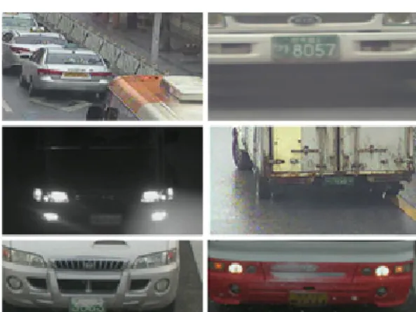
Fig. 1. Examples of bad images for a LPR system
LPD in the video for identifying a vehicle by LPR.We propose an efficient Vehicle-to-LP detection system which is based on motion detection and a cascade of boosted classifiers to make a faster detector. In the first step of this system, motion detection of a frame is used in the vehicle detection.
We can obtain blobs and limited searching regions as candidate areas that means we only classify small sub-windows in candidate regions. The second step is to use the cascade of boosted classifiers for LPD.
By combining two steps, we are able to reduce computational time and keep the performance of cascade of boosted classifiers.
This paper is organized as follows: Problems and challenges are illustrated in Section 2, the proposed LPD system in a fixed camera environment is described in Section 3, and the experimental results in Section 4 show that the proposed system is able to ensure fast LPD as well as achieve the high detection accuracy than other existing systems.
Finally, a conclusion is summarized in Section 5.
Ⅱ. Problems and Challenges
There are a number of possible difficulties available for a LPR system affected by images. All complications are summarized as follows :
(1) Bad image quality (resolution) problem caused by using a low-quality camera or long distance between a camera and a vehicle.
(2) Blurry image problem caused by mainly motion blur.
(3) Illumination and low contrast due to overexposure, reflection or shadows, caused by vehicle headlight or other light sources during the image acquisition.
(4) Occlusion problem, an object obscured or dirt on the LP during the image acquisition.
(5) Partial LP image problem caused by a distorted LP or only some part of LP.
(6) Environmental problems caused by snowing, raining, etc. during the image acquisition.
Fig. 1 shows some examples of difficult images for LPR system.
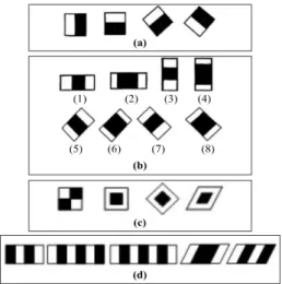
To properly work with LPR systems, we must manage a large variety of LPs, especially in South Korea. Each province in Korea has its own LP color, pattern, and number format and other characters. Different colors represent different types of vehicles. Moreover, there are three different sizes of LPs available in Korea, such as large (520 mm x 110 mm), medium (440 mm x 200 mm), and small (335 mm x 170 mm or 155 mm). Fig. 2 presents the different types and sizes of LPs available in Korea.
Fig. 2. Different types and sizes of Korean LPs
Ⅲ. Vehicle-to-LP detection
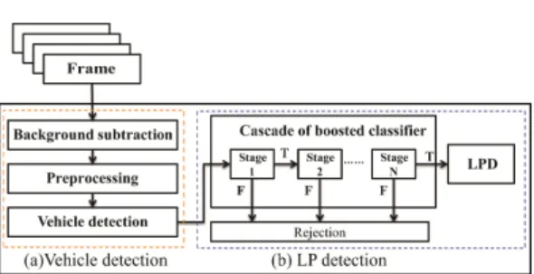
Our proposed LPD system is divided into two phase; vehicle detection and LP detection. In a traffic surveillance system, background subtraction using background model is very useful to detect ROI for LPD under the fixed camera environment.
The first step of our system is vehicle detection which can reduce the computational time since there are few searching areas. Next step is LP detection.
Fig. 3. Vehicle-to-LP detection framework
We are able to apply a trained cascade of boosted classifiers to each ROI for LPD. Fig. 3 demonstrates the proposed Vehicle-to-LP detection framework.
3.1 Vehicle Detection
Detecting a LP in a large area needs much more computational complexity. If we detect the vehicle region as a ROI quickly from an image then the area is reduced for detecting a LP and minimizes computational complexity. Once we know the vehicle region, we can detect the LP promptly. So the vehicle detection is the first and the most important part of our proposed system. We use a GMM and an expectation-maximization (EM) algorithm to identify moving objects regions in our test video and after that using some image preprocessing methods to find the vehicle region as a ROI. The detailed description of our proposed vehicle detection procedure will be given later.
In computer vision, background subtraction using a GMM is often used. The algorithm of background subtraction using a GMM is as follows;
(1) Initialize. Choose the number of Gaussian variables and learning constant : values in the range 0.01-0.1 are commonly used. At each pixel, initialize Gaussian variables
∑ with a mean vector and a covariance matrix ∑and corresponding weights .
(2) Acquire a frame , with an intensity vector
- probably this will be an RGB vector
. Determine which Gaussian variable matches this observation, and select the ‘best' of these as . In an 1-D case, we would expect an observation to be within, say, of the mean. In a multi-dimensional case, a simplifying assumption
is made for computational complexity reason: the different components of the observation are taken to be independent and of equal variance
, allowing a quick test for ‘acceptability'.
(3) If a match is found as a Gaussian variable :
(a) Set the weights according to equation (1), and re-normalize.
≠
(1)
(b) Set
(2)and
(3)
(4)
(4) If no Gaussian variable matches : then determine and delete
. ThenSet
(5)
(The algorithm is reasonably robust to these choices).
(5) Determine
as in equation (6), and thence from the current ‘best match' Gaussian whether the pixel is likely to be foreground or background.
(6)(6) Use some combination of blurring and morphological dilations and erosions to remove very small regions in the difference image, and to fill in
‘holes' etc. in larger ones. Surviving regions represent the moving objects in the scene.
(7) Return to step 2 for the next frame.
A GMM[8] is employed to make background model using more than two Gaussian distributions.
In this method, the background model is statistically modeled on each pixel. In order to adapt to pixel
value changes, we use an adaptive GMM which updates the training set by adding new samples and discarding the old ones. Besides, we can estimate parameters such as weight, mean and covariance by an expectation-maximization (EM) algorithm. The EM algorithm identifies a local maximum, usually of reasonable quality. The EM proceeds iteratively:
At each stage it estimates the influence of each Gaussian variable on each data sample (expectation), and then refines the estimates of the Gaussian parameters (maximization) : If we have (an estimate of) mean and covariance ∑,
we can compute the probability of the Gaussian variable being responsible for as;
(7)
That is, the ratio of the probability of given
( is normal with mean
and covariance ∑ ;
∑ ) to the overall probability of (regardless of the generating a Gaussian variable), suitably weighted by the current . We can then define
(8)
That is, the mean over the data set.
Correspondingly, now we can estimate the improved values of and ∑;
(9)
(10)
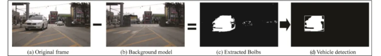
In the next step, the difference between the background model and the current image is evaluated and we find the moving objects regions from our test video as extracted blobs as shown in Fig. 4(c). Morphological processing and connected component are used as preprocessing. Firstly, morphological opening and closing is necessary to use since there are many noises right after background subtraction. The primary morphological operations arc dilation and erosion. Both dilation and erosion are produced by the interaction of a set called a structuring element[8] with a set of pixels of interest in the image. The structuring element has both a shape and an origin. Let
be a set of pixels and let
be a structuring element. Let
be the reflection of
about its origin and followed by a shift by . Dilation, written
⊕
, and Erosion, written
⊖
, is the set of all shifts that satisfy the following:
⊕
∩
⊆
(11)
⊖
⊆
(12)We can combine dilation and erosion to build two important higher order operations:
is said to be opened by
if the erosion of
by
is followed by a dilation of the result by
.
∘
⊖
⊕
(13)Similarly,
is said to be closed by
if
is first dilated by
and the result is then eroded by
. Thus,
∙
⊕
⊖
(14)After using the morphological opening and closing, all noises are eliminated.
Secondly, the foreground regions of each frame are grouped into a connected component and we use blob labeling or connected component analysis (CCA) to detect connected regions in binary digital images[10]. The procedure of CCA as follows;
Assume that the segmented image
consists of Fig. 4. Background subtraction process and vehicle detection
disjoint regions
. The image
often consists of objects and a background.
≠
(15)where
is the set complement,
is considered background, and other regions are considered objects. The input to a labeling algorithm is usually either a binary or multi-level image, where background may be represented by zero pixels , and objects by non-zero values. A multi-level image is often used to represent the labeling result, background being represented by zero values, and regions represented by their non-zero labels. After using the CCA, we can find the connected component as a vehicle ROI and each component is bounded by 2D bounding box. Hence, we are able to obtain vehicle region as shown in Fig. 4(d).3.2 LP Detection
LP detection is the second phase of our proposed system. We use a “cascade” of boosted classifiers for finding a LP region in a vehicle ROI image. To obtain the cascade of boosted classifiers, we chose the most widely used form of boosting algorithm called AdaBoost, short for ‘adaptive boosting’.
Having such a large feature set available together with a training set of
positive and
negative examples (assuming a two-class problem; LP and Non-LP in our case), it is foreseeable that only a small number of these features can be used in combination to yield an effective classifier. The small set of distinguishing features can be selected using the AdaBoost algorithm. A single rectangle feature is first selected using a weak learning approach to best separate the positive and negative examples, followed by additional features identifiedby the iterative boosting process[9]. For each selected feature, the weak learner finds an optimal threshold minimizing the number of misclassified examples from the training set. Each weak classifier is thus based on a single feature and a threshold .
(16)
where is a polarity indicating the direction of the inequality sign and is an image subwindow on which the individual rectangle features are calculated. The AdaBoost feature selection and classifier learning algorithm is described as follows;
(1) Consider a two-class problem (LP and Non-LP), a training set of positive and negative examples , and their corresponding class identifiers ∈ .
(2) Initialize
, the number of features to be identified.(3) Set ; for each sample , initialize weights
(17)
(4) For ≠ , normalize the weights to produce a probability distribution
(18)
(5) For each feature , train a classifier
restricted to using a single feature. Evaluate its
Fig. 5. Background subtraction process and vehicle detection
Fig. 6. Examples of some positive and negative sample images for training module
Fig. 7. Normalized with boundary padding
Fig. 8. Examples of converted and filtered images (a) Positives samples (b) Negative samples
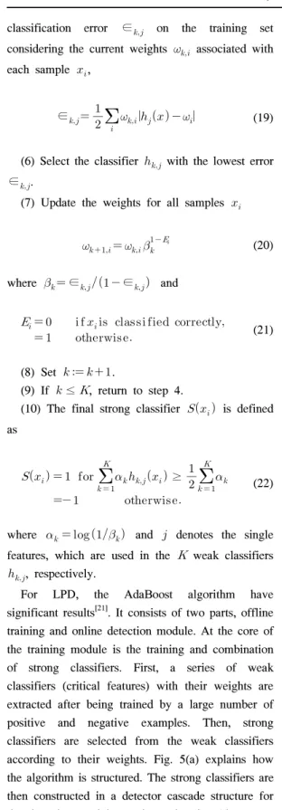
classification error ∈ on the training set considering the current weights associated with each sample ,
∈
(19)
(6) Select the classifier with the lowest error
∈.
(7) Update the weights for all samples
(20)
where ∈ ∈ and
(21)
(8) Set .
(9) If ≤
, return to step 4.(10) The final strong classifier
is defined as
≥
(22)
where and denotes the single features, which are used in the
weak classifiers, respectively.
For LPD, the AdaBoost algorithm have significant results[21]. It consists of two parts, offline training and online detection module. At the core of the training module is the training and combination of strong classifiers. First, a series of weak classifiers (critical features) with their weights are extracted after being trained by a large number of positive and negative examples. Then, strong classifiers are selected from the weak classifiers according to their weights. Fig. 5(a) explains how the algorithm is structured. The strong classifiers are then constructed in a detector cascade structure for the detection module as shown in Fig. 5(b).
For the training module, positive sample images
and negative sample images are required. The positive sample images are LP images only; the negative sample images are background images without an LP image. A total of 15,000 images are used as the positive samples (6,000 large; 3,000 medium; and 6,000 small) and 25,000 images are used for the negative samples for our training experiment. Fig. 6 presents some positive and negative sample images. The AdaBoost training algorithm requires for the positive sample images to be of the same size. For this reason, we must normalize all three types of Korean LP images into one equal size.
For image pre-processing, the image converting[12]
and filtering (Gaussian filter)[13] methods are applied to the training images. The results of image converting and filtering are shown in Fig. 8.
Fig. 9. Haar-like prototypes used in our algorithm (a) Edge features (b) Line features (c) Center-surrounding features (d) Plate character features
Fig. 10. (a) Summed area of integral image (b) Summed area of rotated integral image
LP location procedures classify images based on the value of simple features. These features use the change in contrast values between adjacent rectangular groups of pixels, rather than the intensity values of a pixel. The contrast variances between the pixel groups are used to determine relative light and dark areas. Two or three adjacent groups with a relative contrast variance form a Haar-like feature.
These features are used for the LPD shown in Fig.
9.
By using a transitional depiction of an image, the simple rectangular features of an image are calculated. This is called the integral image[14],[15]. The integral image is an array that contains the sums of the pixel intensity values located directly to the left of a pixel and directly above the pixel at location , inclusive. Therefore, if
is the original image and
is the integral image, the integral image is calculated as shown in equation (3) and demonstrated in Fig. 10.
′≤ ′≤
′ ′(23)
The features are rotated 45 degrees, similar to the line feature shown in Fig. 9.b(5), as presented by Lienhart and Maydt[16]. Such features require another transitional depiction called the rotated integral image or rotated sum auxiliary image. The rotated
integral image is computed by finding the sum of the pixel intensity values that are located at a 45-degree angle to the left and above of the value, and below the value. Therefore, if
is the original image and
is the rotated integral image, the integral image is calculated as shown in equation (24) and illustrated in Fig.10.
′≤ ′≤ ′
′ ′(24)
Integral image is used for fast evaluation of features and the AdaBoost is used for feature selection which chooses the best region suited for detection and construct the rejector-based cascade which is a great method to reduce computational time. The methods used involve training a strong classifier using the AdaBoost algorithm. Over numerous sequences, the AdaBoost chooses the best performing weak classifier from a group of weak classifiers acting on a single feature; once trained, the AdaBoost combines the respective votes of the classifiers in a weighted manner, thus forming a strong classifier. This strong classifier is then applied to the sub-regions of the image that is being scanned for possible LP locations. The weak learning algorithm is designed to select the single rectangle feature that best separates the positive and negative samples. A background threshold of 80, a number of training stages of 14, and a total number of features of 61,789 are used in our AdaBoost training phase.
In the AdaBoost detection module, a window will be considered as a LP if and only of all layers of the detector cascade classifies it as LP. The strong classifiers combine with each other to form a classifier cascade. The strong classifier from the first
Fig. 11. Visualization of Vehicle-to-LP detection
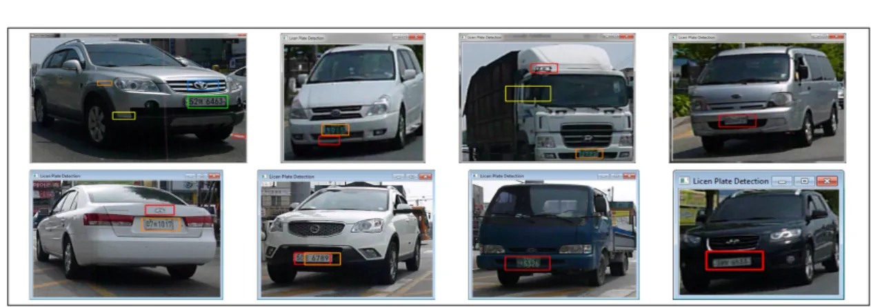
Fig. 12. Successful images for LPD using our proposed system
Fig. 13. Verifying images with CCA and saving LP images
layer allows a vast majority of the image regions to be recognized and passed to the next layer; at the same time, the classifier rejects as many negative samples as possible. Thus, the classifier cascade has stronger classification abilities, and the final result is more likely to be an LP. During the combination process, the strong classifier that consists of more important features and an easier structure is placed at the top of the entire classifier cascade in order for the system to exclude as many negative samples as possible, thus accelerating the detection of LPs. The searching procedure of an AdaBoost cascade classifier is shown in Fig. 5(b). As shown in Fig.
11(c), we apply a cascade AdaBoost as LP detection to each ROI after vehicle detection. Finally, a LP is detected as shown in Fig. 11(d).
There are many false-positives and false-negatives areas detected as LP regions using the cascade of boosted classifier shown in Fig. 12. To ignore such false-positives and false-negatives, we use CCA[10]. Fig. 13 explains the procedure for verifying detected LP images with CCA. The verification procedure of LP and non-LP is as follows;
Algorithm: Procedure Blob (number, area);
1: If number of Blob >= 6 and <=10;
2: area = LP;
3: else
4: area= Non-LP;
5: End.
After justifying LP and Non-LP images; only LP images are accepted for future processing (character recognition) and all Non-LP images are rejected.
Vehicle Detection
Success Failure Time
99.66% 0.34% 18ms
Table 1. Vehicle detection using adaptive GMM
LPD False-positives and
False-negatives
Detection
rate Time
Before applying
CCA
After applying
CCA 99.14% 24ms
12.5% 0%
Table 2. LPD using cascade of boosted classifier.
References Main Procedures for LPD system
Database Size
Image/Frame
resolution LPD Rate Processing
Time Real Time Plate Format [17] Statistical Measures of
License Plate Features 460 images 648×486 pixels 96.4% 0.1s Yes Australian Plates
[18]
License plate features, Vertical edge, morphological operation
345 images 720x486 pixels 98.26% 59ms Yes Greek
Plates
[19] Statistical analysis of
Discrete Fourier Transform 1758 images 640×480 pixels 97.27% 150ms Yes Saudi Plates
[20] Gaussian Windows 595 images 512×240 pixels 98.5% - - Korean
Plates [21] Harr-like and EOH feature 986 images 640×320 pixels 98.41% 45ms Yes Chinese
Plates Our
proposed System
Adaptive GMM and Cascade of Boosted Classifier
10 min
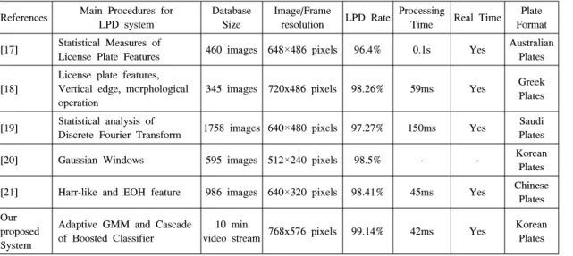
video stream 768x576 pixels 99.14% 42ms Yes Korean Plates Table 3. Comparison of LPD rate and Processing Time
Ⅳ. Experimental Results
To test the LPD using an adaptive GMM and a cascade of boosted classifiers as proposed in this paper, we applied the method to a database of 10 minute video stream with the resolution of 768x576 that were recorded at different times and weather conditions. The experiment is based on the conditions of a system with CPU 3.40-GHz Intel Core i7-2600 and 8.00 GB of RAM, and implemented using Microsoft Visual Studio 2012 with OpenCV library. Table 1 lists the vehicle detection rate and the computational time with the adaptive GMM.
Table 1 lists the vehicle detection rate and time, the percentage of failure rate can be reduce by adjusting the camera position. If we adjust the height of camera from road surface, the occlusion problem can be reduced and the failure rate can also be improved.
Table 2 lists the LPD rate, the percentage of false-positives and false-negatives, and the computational time with a cascade of boosted classifiers. From Table 2, the percentage of detected false-positives and false-negatives are 12.5%.
After applying CCA, no false-positives and false-negatives are remained. Therefore, the overall detection rate (from table 1 and 2) is 99.14% and
the computational time is approximately 42ms. Most of the existing LPD systems are using static images for their experiments (database) but we use real-time video stream for our experiment (database). So many of the existing systems are not real-time and have low processing time, but we have the real-time operation for LPD with very fast processing time.
Comparison of some LPR systems LPD rate and processing time with our system for LPD shows in Table 3.
Ⅴ. Conclusions
We demonstrated a procedure for LPD
algorithms. We used two methods for our LPD system, adaptive GMM and cascade AdaBoost. Our proposed system Vehicle-to-LP detection is separated into two stages, vehicle detection and LPD, which make our proposed system extremely simple and effective for LPD. In this paper, we demonstrated that such simplicity and effectiveness allow our method to provide a better performance than other existing methods. Most of the existing techniques are tremendously complex and are not suitable for real-time applications; however, our proposed algorithm is not complex, thus rendering it suitable for real-time applications. Using our proposed method, the experimental results show that the LPD rate is 99.14% with a computational time of 42ms, which is significantly faster than other existing methods. In regard to our proposed method, practicing and improving its accuracy and practicality are considerations for future work.
Moreover, character recognition in a LP is our principal future work.
References
[1] C. Luis, M. Marco, G. José, and A. Francisco,
“License plate detection using neural networks,” Lecture Notes in Computer Sci., vol. 5518, pp. 1248-1255, Jun. 2009.
[2] X. Wang, H. Li, L. Wu, and Q. Hong,
“Genetic algorithm based neural network for license plate recognition,” Lecture Notes in
Computer Sci., vol. 7951, pp. 391-400, Jul.
2013.
[3] Z. Dong and X. Feng, “Research on license plate recognition algorithm based on support vector machine,” J. Multimedia, vol. 9, no. 2, pp. 253-260, Feb. 2014.
[4] W. Hui, L. Gang, K. Hongchang, and S.
Liufu, “A vehicle license plate detection method based on clustering analysis,” in Proc.
Int. Conf. Computer Science and Service System, pp. 1413-1416, Nanjing, China, Aug.
2012.
[5] P. Viola and M. Jones, “Robust real-time face detection,” Int. J. Computer Vision, vol. 57,
no. 2, pp. 137-154, May 2004.
[6] B. Chung, K. Park, and S. Hwang, “A fast and efficient haar-like feature selection algorithm for object detection,” J. KICS, vol.
38A, no. 6, pp. 486-491, Jul. 2013.
[7] Z. Zivkovic, “Improved adaptive gaussian mixture model for background subtraction,” in
Proc. 17th Int. Conf. Pattern Recognition, vol.
2, pp. 28-31, Washington DC, USA, Aug.
2004.
[8] W. Hu, T. Tan, L. Wang, and S. Maybank,
“A survey on visual surveillance of object motion and behaviors,” IEEE Trans. Systems,
Man, and Cybernetics, PART C: Applications
and Reviews, vol. 34, no. 3, pp. 334-352, Aug. 2004.[9] E. R. Dougherty, An introduction to
morphological Image processing, Tutorial
Texts in Optical Engineering (Book 9), SPIE Optical Engineering Press, 1992.[10] M. Sonka, V. Hlavac, and R. Boyle, Image
processing, analysis, and machine vision,
Thomson Learning, 3rd Ed., Thomson corporation USA, 2008.[11] R. Szeliski, Computer vision: Algorithms and
applications, Texts in Computer Science,
Springer London, 2011.[12] T. Kumar and K. Verma, “A theory based on conversion of RGB image to gray image,” Int.
J. Computer Appl., vol. 7, no. 2, pp. 7-10,
Sept. 2010.[13] D. Forsyth and J. Ponce, Computer vision: A
modern approach, Prentice Hall, 2
nd Ed., Pearson, 2003.[14] P. Viola and M. Jones, “Rapid object detection using a boosted cascade of simple fFeatures,” in Proc. IEEE Computer Soc.
Conf. on Computer Vision and Pattern Recognition, vol. 1, pp. I-511-I-518, Kauai,
HI, USA, Dec. 2001.[15] K. Park and S. Hwang, “An improved normalization method for haar-like features for real-time object detection,” J. KICS, vol. 36C, no. 8, pp. 505-515, Aug. 2011.
[16] R. Lienhart and J. Maydt, “An extended set of
haar-like features for rapid object detection,”
in Proc. IEEE Int. Conf. Image Processing
(ICIP), vol. 1, pp. 900-903, New York, USA,
Sept. 2002.[17] L. Zheng, X. He, B. Samali, and L. T. Yang,
“An algorithm for accuracy enhancement of license plate recognition,” J. Computer Syst.
Sci., vol. 79, no. 2, pp. 245-255, Mar. 2013.
[18] N. Boonsim and S. Prakoonwit, “License plate localization based on statistical measures of license plate features,” Int. J. Recent Trends in
Eng. Technol., vol. 10, no. 1, pp. 38- 45, Jan.
2014.
[19] R. Al-Hmouz and K. Aboura, “License plate localization using a statistical analysis of Discrete Fourier Transform signal,” Computers
& Electrical Eng., vol. 40, no. 3, pp. 982-992,
Apr. 2014.[20] Y. Kang and C. Bae, “License plates detection using a Gaussian windows,” J. KICS, vol.
37A, no. 9, pp. 780-785, Sept. 2012.
[21] S. Xian, L. Shutao, “License plate detection based on improved Real Adaboost,” IEEE Int.
Conf. Veh. Electron. Safety (ICVES), pp.
169-173, Beijing, China, Jul. 2011.
Md. Mostafa Kamal Sarker
He received his B.S. degree from Shahjalal University of Science and Technology, Sylhet, Bangladesh, in 2009, and his M.S. degree from Chonbuk National University, Jeonju, Republic of Korea, in 2013. He is currently doing research to obtain his Ph.D. degree of Electronic Convergence Engineering at Wonkwang University, Iksan, Republic of Korea. His research interests include the areas of image processing, pattern recognition, and computer vision.
Moon Kyou Song
He received the B.S., M.S.
and Ph.D. degrees in Electronics engineering from Korea University, Seoul, Korea, in 1988, 1990, and 1994, respectively. In 1994, he joined the faculty of Wonkwang University, Korea, where he is a Professor in the Department of Electronic Convergence Engineering. He was an Invited Researcher with Electronic Telecommunications Research Institute (ETRI), Daejeon, Korea, from 1997 to 1998 and 2000 to 2001. He was a Visiting professor with University of Victoria, BC, Canada, during 1999-2000 and Stanford University, CA, USA, during 2006-2007. He is a senior member, IEEE.