Reliability estimation and ratio distribution in two independent Pareto-Pareto and power function^†

Reliability estimation and ratio distribution in two independent Pareto-Pareto and power function ^†

Changsoo Lee ¹ · Kyungsu Ahn ²

12 Department of Flight Operation, Kyungwoon University

Received 10 March 2020, revised 26 March 2020, accepted 3 April 2020

Abstract

We consider reliability estimations in two independent Pareto random variables hav- ing different scale parameter, and two independent Pareto and Power function random variables. And then we compare mean squared errors of two reliability estimators for each case. We consider the distribution for the ratio based on two independent Pareto random variables having different scale parameter, and two independent Pareto and Power function random variables respectively. And we observe the skewness for the ratio and study numerically trends for the skewness for the ratio based on two inde- pendent Pareto random variables having different scale parameter and two independent Pareto and Power function random variables.

Keywords: Hypergeometric function, Pareto distribution, Power function distribution, reliability, skewness.

1. Introdunction

An example of some beginning importance is the use of an exponential distribution with a threshold parameter to apply life times of lights and machines.

For independent random variables X and Y , and a real number c, the probability P (X <

c · Y ) is as given in Woo (2006): (i) it is reliability when c = 1, (ii) it is the distribution of the ratio X/(X + Y ) when c = t/(1 − t) for 0 < t < 1.

The reliability will increase the need for the industry to perform the systematic study for identifications and the reduction of causes of failures. These reliability studies must be performed by persons who (a) can identify and quantify the modes of failures, (b) know how to obtain and analyze the statistics of failure occurrences, and (c) can construct math- ematical models of the failure that depend on, for example, the parameters of the material strength or the design quality, the fatigue or the wear resistance, and the stochastic nature of the anticipated duty cycle in Saunders (2007). Ali and Woo (2005) studied the reliability in a power function distribution. Moon and Lee (2009) studied the reliability in the gamma

† This research is supported by 2020 Kyungwoon University Research Fund.

1

Corresponding Author : Associate professor, Department of Flight Operation, Kyungwoon University, Gumi 730-850, Korea. E-mail: [email protected]

2

Assistant professor, Department of Flight Operation, Kyungwoon University, Gumi 730-850, Korea.

case. Lee et al. (2010) studied reliability estimations and the density function of the ratio in right truncated Rayleigh distributions. Ali et al. (2010) studied estimations of the reliability P (Y < X) when X and Y belong to different distribution families, and Yoon and Lee (2012) studied reliability estimations and the distribution of the ratio in two independent variables with different distributions. Zaka and Akhter (2014) considered the modified moment, the maximum likelihood and percentile estimators for the parameters of the Power function distribution.

We consider reliability estimations in two independent Pareto random variables having dif- ferent scale parameters, and two independent Pareto and Power function random variables.

And then we compare mean squared errors of two reliability estimators for each case. We consider the distribution for the ratio based on two independent Pareto random variables having different scale parameter, and two independent Pareto and Power function random variables, respectively. And we observe the skewness for the ratio and study numerically trends for the skewness for the ratio based on two independent Pareto random variables having different scale parameter and two independent Pareto and Power function random variables

2. Pareto distribution

2.1. Estimating reliability

Let X and Y be two independent Pareto random variables each having the density function (2.1) with different scale parameters β 1 and β 2 and known parameter α, respectively:

f X (x) = αβ ₁ ^α /x ^α+1 , x > β 1 > 0, α(> 0) and

f _Y (y) = αβ ₂ ^α /y ^α+1 , y > β ₂ > 0, α(> 0). (2.1) In this section, we consider the case for the estimation of P (Y < X) when (X, Y ) is a pair of two independent Pareto random variables. As an application of this case, X and Y are representing two kinds of the income and the consumption in the economy.

Now, we consider the reliability R(ρ) = P (Y < X) as following:

Proposition 2.1 Let X and Y be independent Pareto random variables each having the density function (2.1) with different scale parameters β 1 and β 2 and known parameter α, respectively. Then

(a) The reliability R(ρ) =

( ρ ^α /2, if 0 < ρ < 1,

1 − ρ ^−α /2, if ρ ≥ 1 , where ρ = β ₁ /β ₂ .

(b) The reliability R(ρ) is a monotone increasing function of ρ.

Proof

(a) For β ₁ < β ₂ , R(ρ) = P (Y < X) = R ∞

β

P (Y < x)f _X (x)dx = ¹ ₂ (β ₁ /β ₂ ) ^α . And also, for β 1 > β 2 , R(ρ) = R ∞

β

P (Y < x)f X (x)dx = 1 − ¹ ₂ (β 2 /β 1 ) ^α .

(b) Since _dρ ^d R(ρ) > 0, R(ρ) is a monotone increasing function of ρ.

Since the reliability R(ρ) is a monotone function of ρ, the inference on R(ρ) is equivalent to the inference on ρ (McCool, 1991). Therefore, it is sufficient for us to consider the estimation of ρ instead of estimating R(ρ).

Assume X 1 , · · · , X n and Y 1 , · · · , Y m be independent random samples from the density function (2.1) each having different scale β ₁ and β ₂ , respectively. Then well-known estimators of β ₁ and β ₂ are given in Johnson et al. (1974) as follows:

β ˆ ₁ = X _(1;n) = X ₍₁₎ and ˆ β ₂ = Y _(1;m) = Y ₍₁₎ . (2.2) From (2.2), the MLE of ρ is

ˆ

ρ = X ₍₁₎ /Y ₍₁₎ . (2.3)

The following density functions are well-known in Rohatgi (1976) as:

f X

(x) = nαβ ₁ ^nα x ^−nα−1 , x > β 1

and

f _Y

(y) = mαβ ^mα ₂ y ^−mα−1 , y > β ₂ . (2.4) From the results (2.4), and formula 3.381(3) in Gradshteyn and Ryzhik (1965), we can obtain the expectation and the variance for the MLE ˆ ρ of ρ = β 1 /β 2 ;

E( ˆ ρ) = nmα ²

(nα − 1)(mα + 1) · ρ and

V ar( ˆ ρ) = [ nmα ²

(nα − 2)(mα + 2) − n ² m ² α ⁴

(nα − 1) ² (mα + 1) ² ]ρ ² , nα > 2. (2.5) From the expectation in (2.5), an unbiased estimator ˜ ρ of ρ is given as:

˜

ρ = (nα − 1)(mα + 1) nmα ² · X (1)

Y ₍₁₎ ,

which it has the variance as follows:

V ar( ˜ ρ) = [ (nα − 1) ² (mα + 1) ²

nmα ² (nα − 2)(mα + 2) − 1]ρ ² , nα > 2. (2.6) From the results (2.5) and (2.6), we can obtain mean squared errors(MSE‘s) of the MLE ˆ

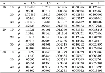
ρ and an unbiased estimator ˜ ρ for ρ ≡ β 1 /β 2 as given in Table 2.1.

Table 2.1 MSE‘s of the MLE ˆ ρ and an unbiased estimator ˜ ρ (units: ρ

)

n m α = 1/4 α = 1/2 α = 1 α = 2 α = 4

10 10 ρ ˆ 1.29683 .10714 .021465 .0050885 .00125548

˜

ρ .96000 .09714 .020938 .0050568 .00125350 20 ρ ˆ 1.79365 .11616 .019965 .0042858 .00100006

˜

ρ .85143 .07556 .014801 .0033747 .00081043 30 ρ ˆ 2.00619 .12684 .021337 .0045182 .00104602

˜

ρ .82526 .07085 .013555 .0030473 .00072624 20 10 ρ ˆ .14021 .04101 .012050 .0033358 .00088248

˜

ρ .16148 .04143 .011134 .0029321 .00075553 20 ρ ˆ .10714 .02146 .005088 .0012555 .00031284

˜

ρ .09714 .02094 .005056 .0012535 .00031270 30 ρ ˆ .10991 .01961 .004315 .0010212 .00024895

˜

ρ .08164 .01647 .003822 .0009289 .00022857 30 10 ρ ˆ .10922 .03846 .011979 .0033929 .00090669

˜

ρ .11529 .03385 .009534 .0025607 .00066590 20 ρ ˆ .05095 .01349 .003583 .0013065 .00023764

˜

ρ .05351 .01350 .003466 .0008828 .00022307 30 ρ ˆ .04036 .00917 .002239 .0005566 .00013895

˜

ρ .03862 .00907 .002233 .0005562 .00013893

As Table 2.1 is observed, because the inference on R(ρ) is equivalent to the inference on ρ in McCool (1991), we obtain the following:

Fact 2.1 Assume X 1 , ·, X n and Y 1 , · · · , Y m be independent random samples from the density function (2.1) each having different scales β 1 and β 2 and known parameter α, re- spectively. Then for ρ ≡ β 1 /β 2 ,

(a) when α = 1, 2 and 4, an estimator R( ˜ ρ) of the reliability R(ρ) = P (Y < X) performs better than the MLE R( ˆ ρ) in the sense of MSE.

(b) when α = 1/2 and 1/4, two estimators can not dominate each other in the sense of MSE.

From the result (b) in Fact 2.1, because the MLE and an unbiased estimator for ρ can not dominate each other in the sense of MSE, a bias estimator ¯ ρ having minimum MSE‘s among {s · X ₍₁₎ /Y ₍₁₎ |s > 0} is recommended as the following:

If there exists satisfying min s>0 E[(s · ^X _Y

(1)

− ρ) ² ] = E[(s 0 · ^X _Y

(1)

− ρ) ² ], then from the expectation and the variance of ˆ ρ in (2.5),

s ₀ = (nα − 2)(mα + 2)

(nα − 1)(mα + 1) if nα > 2.

Therefore, ¯ ρ = (nα−2)(mα+2) (nα−1)(mα+1) · ^X _Y

(1)

has the minimum MSE among a family n s · ^X _Y

(1)

|s > 0 o . And then, because the inference on R(ρ) is equivalent to the inference on ρ in McCool (1991), we can obtain the following:

Corollary 2.1 Under the same conditions of Fact 2.1, the reliability estimator R( ¯ ρ) performs better than other two estimators R( ˆ ρ) and R( ˜ ρ) in the sense of MSE regardless of α−values.

Now, we consider an interval estimation of ρ = β 1 /β 2 .

From the quotient density in Rohatgi (1976), the density function of a pivot quantity P ≡ ρ · Y ₍₁₎ /X ₍₁₎ is derived as:

f _P (x) = ( _mnα

(m+n) x ^nα−1 , 0 < x < 1,

mnα

(m+n) x ^−mα−1 , x ≥ 1.

And then for given p _i ≥ 0 (i = 1, 2) with 0 < 1 − p 1 − p 2 < 1,

([p ₁ (1 + n/m)] ^1/(nα) · X ₍₁₎ /Y ₍₁₎ , [p ₂ (1 + m/n)] ^−1/(mα) · X ₍₁₎ /Y ₍₁₎ ) is an (1 − p ₁ − p ₂ )100% conservative confidence interval for ρ = β ₁ /β ₂ .

2.2. Distribution of the ratio

In this section, we consider the ratio R _X = X/(X + Y ), when X and Y are independent Pareto random variables each having density function (2.1) with different parameters β ₁ and β ₂ anf known parameter α, respectively. First, from the quotient density in Rohatgi (1976) and the integration, we can derive the quotient density Q = Y /X as follows: For ρ = β ₁ /β ₂ ,

f Q (x) = ( _α

2 ρ ^−α x ^−α−1 , if x ≥ ρ ⁻¹ ,

α

2 ρ ^α x ^α−1 , if 0 < x < ρ ⁻¹ . (2.7) From the quotient density function (2.7), we can derive the density function of the ratio R _X = X/(X + Y ) as follows:

f R

(r) = ( _α

2 ρ ^−α r ^α−1 /(1 − r) ^α+1 , if 0 < r ≤ ρ/(1 + ρ),

α

2 ρ ^α (1 − r) ^α−1 /r ^α+1 , if ρ/(1 + ρ) < r < 1. (2.8) From the result (2.8) and formula 3.194 (1) in Gradshteyn and Ryzhik (1965), we can obtain k−th moments of the ratio R _X as follows:

For k = 1, 2, · · · ,

E(R ^k _X ) = 1

2 ² F ₁ (k, α; α + 1; ‘ − 1/ρ) + α

2(k + α) ρ ^k ₂ F ₁ (k, k + α; k + α + 1; −ρ), (2.9)

where ₂ F ₁ (a, b; c; x) is the hypergeometric function.

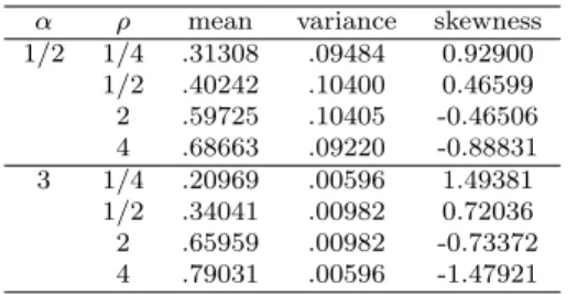
Based on k−th moments of the ratio R _X , and by recursion formulas 15.2.13 and 15.2.25 of the hypergeometric function and formula 15.1.8 in Abramowitz and Stegun (1970), we can obtain means, variances and coefficients of the skewness as given in Table 2.2.

Table 2.2 Mean, variance and coefficient of skewness for the density (2.8) α ρ mean variance skewness

1/2 1/4 .31308 .09484 0.92900 1/2 .40242 .10400 0.46599 2 .59725 .10405 -0.46506 4 .68663 .09220 -0.88831 3 1/4 .20969 .00596 1.49381 1/2 .34041 .00982 0.72036 2 .65959 .00982 -0.73372 4 .79031 .00596 -1.47921

From Table 2.2, we can observe the following trends:

Fact 2.2 When X and Y are independent Pareto random variables each having density function (2.1) with different parameters β ₁ and β ₂ and known parameter α, respectively.

For α = 1/2 and 3, the density function of the ratio R _X = X/(X + Y ) is right skewed when ρ = β 1 /β 2 = 1/4 and 1/2, but it is left skewed when ρ = 2 and 4.

3. Pareto and power function distributions

3.1. Estimating reliability

Assume X and Y be two independent Pareto random variable having density function (2.1) with unknown parameter β and known parameter α and a Power function random variable having density function (3.1) with θ(> β) and known δ(6= α) > 0, respectively.

f _Y (y) = (δ/θ ^δ )y ^δ−1 , 0 < y < θ, δ > 0, (3.1) As the consideration of Ali et al. (2010), we consider the case for estimations of the reliability P (Y < X) when (X, Y ) is a pair of Pareto and Power function random variables, respectively. As an application of this case Y , representing time to sustain a proper level of the radioactivity, is a Power function random variable and X, representing keeping up the time of a white rat from its beginning time which is exposed to the radioactivity, is a Pareto random variable in Saunders (2007).

Now, we consider the reliability R(η) = P (Y < X) as following:

Proposition 3.1 Assume X and Y be two independent Pareto random variable having density function (2.1) with β > 0 and known α > 0 and a Power function random variable having density function (3.1) with θ(> β) and known δ(6= α) > 0, respectively. Then

(a) the reliability R(η) = _δ−α ^δ η ^α − _δ−α ^α η ^δ , η ≡ β/θ < 1, α 6= δ.

(b) the reliability R(η) is a monotone decreasing function of η.

Proof

(a) R(η) = P (Y < X) = Z ∞

β

P (Y < x)f X (x)dx

= Z θ

β

P (Y < X)f _X (x)dx + Z ∞

θ

f _X (x)dx = α

δ − α [(β/θ) ^α − (β/θ) ^δ ] + (β/θ) ^α . (b) Since _dη ^d R(η) = _δ−α ^δα (η ^α−1 − η ^δ−1 ) < 0 for 0 < η < 1, and hence we have done.

Since the reliability R(η) is a monotone function of η, the inference on R(η) is equivalent to the inference on η (McCool, 1991). Therefore, it is sufficient for us to consider estimations of η instead of estimating R(η).

Assume X ₁ , · · · , X _n and Y ₁ , · · · , Y _m be independent random samples from the density function (2.1) with β > 0 and known α > 0 and a Power function random variable having density function (3.1) with θ(> β) and known δ(6= α) > 0, respectively.

Then for known α and δ, the following well-known estimators of β and θ are given in Johnson et al. (1974) as:

β = X ˆ _(1;n) = X ₍₁₎ and ˆ θ = Y _(m;m) = Y _(m) . (3.2) From the result (3.2), a MLE ˆ η of η is given by:

ˆ

η = ˆ β/ˆ θ = X ₍₁₎ /Y _(m) . (3.3)

From the density function of X ₍₁₎ in (2.4) and the density function of Y _(m) as the following

f Y

(x) = (mδ/θ ^mδ )x ^mδ−1 , 0 < x < θ, we can obtain the expectation and variance the a MLE ˆ η of η as follows:

E(ˆ η) = nmαδ

(nα − 1)(mδ − 1) · η and

V ar(ˆ η) = [ nmαδ

(nα − 2)(mδ − 2) − n ² m ² α ² δ ²

(nα − 1) ² (mδ − 1) ² ]η ² , mδ > 2, nα > 2. (3.4) From the expectation in (3.4), an unbiased estimator ˜ η of η is given as:

˜

η = (nα − 1)(mδ − 1)

nmαδ · X (1) /Y (m) ,

which it has the variance as follows:

V ar(˜ η) = [ (nα − 1) ² (mδ − 1) ²

nmαδ(nα − 2)(mδ − 2) − 1]η ² , mδ > 2, nα > 2. (3.5)

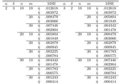
Table 3.1 MSE‘s of a MLE ˆ η and an unbiased estimator ˜ η (units: η

)

α δ n m MSE α δ n m MSE

2 3 10 10 η ˆ .012618 3 2 10 10 η ˆ .012618

˜

η .003972 η ˜ .003972

20 η ˆ .008479 20 η ˆ .005804

˜

η .003066 η ˜ .001849

30 η ˆ .007446 30 η ˆ .004342

˜

η .002904 η ˜ .001478

20 10 η ˆ .005804 20 10 η ˆ .008479

˜

η .001849 η ˜ .003066

20 η ˆ .002879 20 η ˆ .002879

˜

η .000945 η ˜ .000945

30 η ˆ .002225 30 η ˆ .001783

˜

η .000784 η ˜ .000575

30 10 η ˆ .004342 30 10 η ˆ .007446

˜

η .001478 η ˜ .002904

20 η ˆ .001783 20 η ˆ .002225

˜

η .000575 η ˜ .000784

30 η ˆ .001243 30 η ˆ .001243

˜

η .000414 η ˜ .000414

From the results (3.4) and (3.5), we can obtain mean squared errors (MSE‘s) of the ML estimator and an unbiased estimator ˜ η of η as given in Table 3.1.

As Table 3.1 is observed, because inference on R(η) is equivalent to inference on η in McCool (1991), we obtain the following:

Fact 3.1 Assume X ₁ , · · · , X _n and Y ₁ , · · · , Y _m be independent random samples from the density function (2.1) with β > 0 and known α > 0 and a Power function random variable having density function (3.1) with θ(> β) and known δ(6= α) > 0, respectively.

Then for η = β/θ < 1, an estimator R(˜ η) of the reliability R(η) = P (Y < X) performs better than a MLE R(ˆ η) in the sense of MSE only when (α, δ) = (2, 3) and (3, 2).

By similar manner as like Corollary 2.1 in Section 2, we can obtain the following bias estimator ¯ η of η = β/θ: For nα > 2 and mδ > 2,

¯

η = (nα − 2)(mδ − 2) (nα − 1)(mδ − 1) · X ₍₁₎

Y _(m) has a minimum MSE among a family {s · ^X _Y

(m)

|s > 0}. And then we can obtain the following:

Corollary 3.1 Under the same conditions of Fact 3.2, the reliability estimator R(¯ η)

performs better than other two estimators R(ˆ η) and R(˜ η) in the sense of MSE regardless of

(α, δ)−values.

Now, we consider an interval estimation of η = β/θ < 1. From quotient density in Rohatgi (1976), the density of a pivot quantity Q ≡ η · Y _(m) /X ₍₁₎ is derived as:

f Q (x) = αδnm

δm − αn [x ^αn−1 − x ^δm−1 ], 0 < x < 1 and mδ 6= nα.

Then the distribution function F _Q (x) of a pivot quantity Q ≡ η · Y _(m) /X ₍₁₎ is given by:

F _Q (x) = αδnm δm − αn [ x ^αn

αn − x ^δm

δm ], 0 < x < 1 and mδ 6= nα.

And for given 0 < γ < 1,

(F _Q ⁻¹ (γ/2) · X ₍₁₎ /Y _(m) , F _Q ⁻¹ (1 − γ/2) · X ₍₁₎ /Y _(m) ) is an (1 − γ)100% confidence interval for η = β/θ.

Remark 3.1 For given 0 < p < 1, there exists x = F _Q ⁻¹ (p) such that p = _δm−αn ^αδnm [ ^x _αn

−

x

δm ], and then an approximate root x of h(x) = δmx ^αn − αnx ^δm − (δm − αn)p = 0 can be solved by using the polynomial function or the bisection method in PROC IML in SAS- Studio.

3.2. Distribution of the ratio

In this section, we shall consider the ratio R X = X/(X + Y ), when X and Y are two independent Pareto random variable having density function (2.1) with β > 0 and known α > 0 and a Power function random variable having density function (3.1) with θ(> β) and known δ(6= α) > 0, respectively.

From the quotient density in Rohatgi (1976), we can derive the quotient density function of V = Y /X as follows: For η = β/θ < 1,

f V (x) = αδ

δ − α [η ^α x ^α−1 − η ^δ x ^δ−1 ], 0 < x < 1/η. (3.6) From the quotient density function (3.6), we can derive the density function of the ratio R X = X/(X + Y ) as follows:

f R

(x) = αδ

δ − α [η ^α (1 − r) ^α−1 /r ^α+1 − η ^δ (1 − r) ^δ−1 /r ^δ+1 ], η

1 + η < r < 1. (3.7)

From the density function (3.7) of the ratio R _X = X/(X + Y ) and a formula 3.194(1)

in Gradshteyn and Ryzhik (1965), the k−th moment of R _X is obtained as follows: For

k = 1, 2, · · · ,

E(R _X ^k ) = δ δ − α ( η

1 + η ) ^α ₂ F ₁ (α − k + 1, α; α + 1; 1 1 + η )

− α

δ − α ( η

1 + η ) ^δ 2 F 1 (δ − k + 1, δ; δ + 1; 1/(1 + η)), (3.8) where 2 F 1 (a, b; c; x) is the hypergeometric function.

Based on k−th moments in (3.8), and by recursion formulas 15.2.13 and 15.2.25 of hy- pergeometric function and formula 15.1.8 in Abramowitz and Stegun (1970), we can obtain means, variances and coefficients of skewness for the ratio density function f _R

(x) in (3.7) as given in Table 3.2.

Table 3.2 Mean, variance and coefficient of skewness of the density (3.7) α δ η mean variance skewness

1/2 1 1/8 .59525 .08637 -0.03352 1/6 .64116 .07135 -0.17965 1/4 .70546 .05694 -0.37833 1/2 .80123 .03305 -0.72037 2/3 .83491 .02522 -0.93295 4 1/8 .47693 .08139 0.51347 1/6 .52611 .07568 0.36926 1/4 .59743 .06457 -0.07433 1/2 .71573 .04146 -0.13271 2/3 .76027 .03239 -0.27232 3 2 1/8 .23701 .01381 1.97071 1/6 .28830 .01598 1.68624 1/4 .37058 .01798 1.34109 1/2 .52812 .01692 0.87536 2/3 .59426 .01488 0.72154 5 1/8 .18244 .00445 2.42502 1/6 .22773 .00570 2.13402 1/4 .30377 .00735 1.77460 1/2 .45996 .00849 1.25907 2/3 .52937 .00892 1.12217

From Table 3.2, we observe the following trends:

Fact 3.2 Assume X and Y are two independent Pareto random variable having density function (2.1) with β > 0 and known α > 0 and a Power function random variable having density (3.1) with θ(> β) and known δ(6= α) > 0, respectively. Then the density function of R _X = X/(X + Y ) is right skewed when η = β/θ = 1/8, 1/6, 1/4, 1/2, 2/3 for (α, δ) = (3, 2) and and η = 1/8 and 1/6 for (α, δ) = (1/2, 4), but it is left skewed when (α, δ, η) has other values in Table 3.2.

Remark 3.2 The consideration in Yoon and Lee (2012) is a special case of that in Section

3.

4. Concluding remarks

In this study, we have proposed estimators for the reliability in two independent Pareto random variables having different scale parameters, and two independent Pareto and Power function random variables. And then we compared mean squared errors of two reliability estimators for each case.

We have obtained the distribution for the ratio based on two independent Pareto random variables having different scale parameter, and two independent Pareto and Power function random variables, respectively. And we have observed the skewness for the ratio and have study numerically trends for the skewness for the ratio based on two independent Pareto random variables having different scale parameter and two independent Pareto and Power function random variables.

References

Abramowitz, M. and Stegun, I. A. (1970). Handbook of Mathematical Functions, Dover Publications Inc., New York.

Ali, M. M., Pal, M. and Woo, J. (2010). Estimation of P (Y < X) when X and Y belong to different distribution families. Journal of Probability and Statistical Science, 8, 19-33.

Ali, M. M. and Woo, J. (2005). Inferences on reliability P (Y < X) in a power function distribution. Journal of Statistics & Management Systems, 8, 681-686.

Gradshteyn, I. S. and Ryzhik, I. M. (1965). Table of integrals, series, and product , Academic Press, New York.

Johnson, N. L., Kotz, S. and Balakrishnan, N. (1994). Continuous univariate distributions, John Wiley &

Sons, New York.

Lee, J. C. and Lee, C. S. (2010). Reliability and ratio in a right truncated Rayleigh distribution. Journal of the Korean Data & Information Science Society, 21, 195-200.

McCool, J. I. (1991). Inference on P (Y < X) in the Weibull case. Communications in Statistics-Simulations, 20, 129-148.

Moon, Y. G. and Lee, C. S. (2009). Inference on reliability P (Y < X) in the gamma case. Journal of the Korean Data & Information Science Society, 20, 219-223.

Rohatgi, V. K. (1976). An introduction to probability theory and mathematical statistics, John Wiley &

Sons, New York.

Saunders, S. C. (2007). Reliability, life testing, and prediction of service lives, Springer, New York.

Yoon, S. U. and Lee, C. S. (2012). Estimating the reliability and distribution of ratio in two independent variables with different distributions. Journal of the Korean Data & Information Sciences Society, 23, 1017-1025.

Woo, J. (2006). Reliability P (Y < X), ratio X/(X + Y ) and skewed-symmetric distribution of two inde- pendent random variables. Proceedings of the Korean Data & Information Science Society, 17,37-42.

Zaka, A. and Akhter, A. S. (2014). Modified moment, maximum likelihood and percentile estimators for the

parameters of the power function distribution. Pakistan Journal of Statistics and Operation Research,

10, 361-368.