반도체디스플레이기술학회지 제18권 제2호(2019년 6월) Journal of the Semiconductor & Display Technology, Vol. 18, No. 2. June 2019.
Modeling with Thin Film Thickness using Machine Learning
Dong Hwan Kim
*, Jeong Eun Choi
*, Tae Min Ha
*and Sang Jeen Hong
*†*†
Department of Electronics Engineering, Myongji University
ABSTRACT
Virtual metrology, which is one of APC techniques, is a method to predict characteristics of manufactured films using machine learning with saving time and resources. As the photoresist is no longer a mask material for use in high aspect ratios as the CD is reduced, hard mask is introduced to solve such problems. Among many types of hard mask materials, amorphous carbon layer(ACL) is widely investigated due to its advantages of high etch selectivity than conventional photoresist, high optical transmittance, easy deposition process, and removability by oxygen plasma. In this study, VM using different machine learning algorithms is applied to predict the thickness of ACL and trained models are evaluated which model shows best prediction performance. ACL specimens are deposited by plasma enhanced chemical vapor deposition(PECVD) with four different process parameters(Pressure, RF power, C
3H
6gas flow, N
2gas flow). Gradient boosting regression(GBR) algorithm, random forest regression(RFR) algorithm, and neural network(NN) are selected for modeling. The model using gradient boosting algorithm shows most proper performance with higher R-squared value. A model for predicting the thickness of the ACL film within the above- mentioned conditions has been successfully constructed.
Key Words : Modeling, Machine learning, Amorphous carbon layer, Film thickness, Box-Behnken
1. Introduction
1In the production environment of semiconductor factories, the monitoring system has been developed, and the collection of historical data of process information of equipment and quality characteristics is complete [1].
Hence, advanced process control(APC) has been gaining more and more relevance in semiconductor manufacturing, thanks to the increase of data volume and computational capabilities [2]. To increase productivity and improve performance of devices, semiconductor industry progresses to reduce the size of device. Accordingly, new fabrication technologies have been developed and researched. In this process, lot of time, cost, strict process condition and resources are required [3]. However, using virtual metrology helps save the time and resources by reducing real manufacturing. Virtual metrology(VM), one of APC techniques, is a method to predict characteristics of manufactured films using machine learning. In practice, there have been many researches to predict characteristics using data of etch, deposition process and data required
†
E-mail: [email protected]
through a variety of sensors [1, 4-6]. As the semiconductor manufacturing
process becomes more complex and the acceptable range of critical
dimension(CD) becomes narrower, VM is a key to achieve high product
quality by providing information based on the metrology result to adjust
tool settings because a small change of a tool setting during process may
cause a significant loss of the final yield [7]. Also, with miniaturization of
semiconductor devices and increasing pattern density of the very large
scale integrated(VLSI) circuit, a single photoresist mask is no longer
applicable for fine line patterning and contact [8]. Memory device has a
capacitor to store charge and its size was getting small. To guarantee
device's performance, capacitor had to compose short width and long
length. Etch fabrication have proceeded high aspect ratio dielectric etch to
satisfy this requirement. Conventional photo resist was no longer fulfill etch
condition because it is soft and has poor selectivity about etch. So hard
mask was introduced to solve such problems. Among many types of hard
mask materials, Amorphous Carbon Layer(ACL) is widely investigated
due to its advantages of high etch selectivity over a photoresist, high optical
transmittance, easy deposition, and removability by oxygen plasma, like
that of a remaining photoresist, after etching [8]. For realizing VM,
machine learning is used to modeling. The use of machine learning is an
Modeling with Thin Film Thickness using Machine Learning 49
advantageous in that it does not involve any assumptions and that the predictive model can be constructed in an easy and fast way [5].
In this study, virtual metrology using different machine learning algorithms(gradient boosting, random forest, neural network) is applied to predict the deposition rate of ACL through plasma enhanced chemical vapor deposition(PECVD) and learned model are analyzed which model is most proper about ACL thickness data.
2. Background 2.1 Machine Learning Algorithm
There are various algorithms for modeling with its advantage and disadvantage. Among them, modeling using neural network has been widely researched [1, 4-5, 9-10].
Neural network has an advantage that it adapts well to training data, but it doesn’t handle missing values and takes long training time [11].
However, ensemble tree method has advantages of handling missing value, obtaining finer-grain and generalized prediction model [11]. Thus, modeling is carried out using neural network and ensemble tree(random forest algorithm and gradient boosting algorithm).
2.1.1 Random forest regression(RFR) algorithm
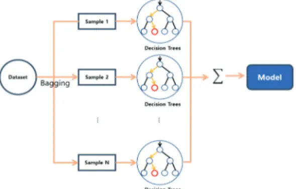
In Fig. 1, RFR algorithm uses a bagging technique with unpruned decision trees. Bagging is a method of generating multiple bootstrap data for given training data, modeling them using each bootstrap data and combining them to calculate the final prediction model. Bootstrap refers to multiple specimens of the same size from raw data through random sampling. Thus, the RFR algorithm prediction for a new observation is made by averaging the output of the ensemble of decision trees.
Fig. 1. Structure of random forest algorithm
2.1.2 Gradient boosting regression(GBR) algorithm Before understanding GBR algorithm, concept of boosting should be known. In machine learning, boosting refers to a way to create a more
accurate and stronger learner by combining relatively inaccurate weak learners. In other words, in Fig. 2, the gradient boosting algorithm refers to a boosting technique in which a plurality of weak prediction models is generated step by step based on the slope of the loss function, and then combined with an ensemble method to have a strong prediction power.
Once the accuracy is low, the first tree model is created, and the second tree model complements the revealed weakness(prediction error). In this way, we continue to supplement weaknesses in the following tree model, and eventually build a strong learning machine.
Fig. 2. Structure of gradient boosting algorithm
2.1.3 Neural Network(NN)
A NN consists of an input layer, hidden layers, and an output layer which has many neurons. The left side of Fig. 3 shows how each neuron works. Each input is multiplied by a weight before entering the neuron.
The multiplied inputs are added as output and goes through an activation function that decides whether to activate the output value. Typical activation functions are Sigmoid, ReLU function. After these activation function, the final output becomes the input of the next neuron. At the right side of Fig. 3, this mechanism occurs in all neurons and each layer is fully connected. The performance of NN may vary depending on the number of hidden layers and the number of neurons. So, it is important to choose optimum number of layers and neurons.
Fig. 3. Structure of neural network
Dong Hwan Kim and Jeong Eun Choi and Tae Min Ha and Sang Jeen Hong 50
2.2 Evaluation method
Although there are several methods to evaluate the modeling, it is wrong to evaluate the modeling with only one method in terms of its reliability. So, in this study, trained models are compared with three of different analysis methods which model is most proper about ACL data in given parameter ranges. To evaluate each model, root mean square error(RMSE), mean absolute percentage error(MAPE) and R-squared, which measure of prediction accuracy of a forecasting method, are used.
2.2.1 RMSE
RMSE is a measure of the differences between values predicted by a model and the values observed.
1
is the number of test data set for model`s validation, y is the value measured through experiments and y is the value measured through the model.
2.2.2 MAPE
MAPE method which is similar with RMSE method, measures the different of real value ( and predicted value ( ), it utilizes absolute value instead of squared value.
|
2.2.3 R-squared
R-squared represents the proportion of the variance for a dependent variable that's explained by an independent variable or variables in a regression model.
1
=
explained variation, = total variation
,
3. Experiments
3.1 Deposition process and data acquisition There are many parameters that influence the film thickness. At this
time, changing all process parameter relevant to film thickness one by one needs a lot of time and inefficient. Also, it may contain meaningless data. So, to plan efficient process parameter value before fabrication and acquire valuable ACL film data, Box-Behnken method of design of experiment(DOE) utilize. Box-Behnken refers to analyze the data statistically and plan to obtain the maximum information with the minimum number of experiments [12]. Through the Box-Behnken method, at least 27 experiments are suggested using four factors(pressure, RF power, gas flow, gas flow. The reason for setting these four factors is that plasma is very sensitive to the above factors and the state of the plasma in PECVD results in a change in the process characteristics. The 27 process recipes derived using the Box- Behnken method is shown in Table 1.
Table 1. Process recipe
Type Value Unit
Electrode gap 1.5 ㎝
Temperature 300 ℃
Time 300 s
Power 230, 250, 270 W
Pressure 800, 1000, 1200 mTorr
gas flow 60, 80, 100 sccm
gas flow 30, 40, 50 sccm
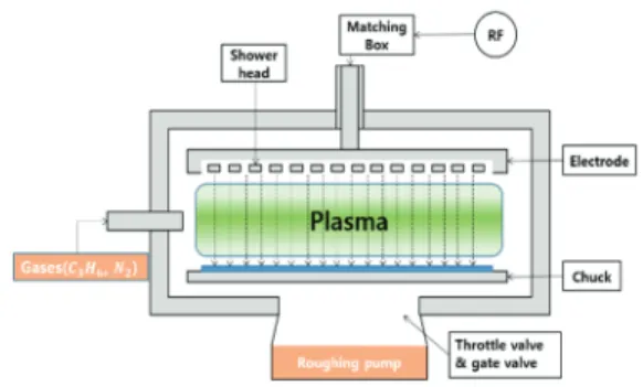
Using established ACL process recipes, film data is acquired by PECVD which has merit of operating at lower temperature than other deposition equipment because it uses plasma.
Fig. 4. Structure of PECVD
As shown in Fig. 4, the two gases are injected through the gas line to
side of the chamber, not through the showerhead. Therefore, there is a
limitation that the injected gases may not spread uniformly. The
thickness of the deposited films was measured by an optical measuring
instrument called a reflectometer.
Modeling with Thin Film Thickness using Machine Learning 51
3.2 Normalization
In order to effectively learn the model using the acquired data, preprocessing of the data is indispensable. If the model is learned by using the data without normalization, the standard deviation is too large for effective learning and training the neural networks would have been very slow because the figure of cost function will be elongated [13].
Normalization was done by the following equation and Table 2. is the normalized total data.
Table 2. Normalization of 27 deposition runs
To train the model, 21 of randomly collected training data is used, and 6 of test data is used to verify the reliability of the models.
4. Result & Discussion
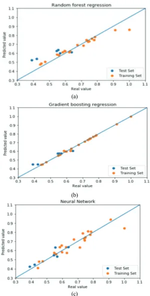
Using normalized thickness data, modeling is done by using different algorithms. In each algorithm, there are various parameters that determine the performance of the model. In case of the RFR in Fig 5(a), the number of trees that are sampled through bagging is specified as 200.
Decision tree constitute of internal nodes which have child node and leaf node. At this time, the minimum number of samples required to split an internal node is set by 2 and the maximum depth of the tree is until all leaves are pure.
In Fig 5(b), the number of samples to be continuously learned through the weak learner is set to 500, and the learning rate was set to 0.01. The number of maximum depth of tree mentioned above was limited to 10.
In the case of NN, Fig 5(c), the parameters of the algorithm used for modeling are 4 hidden layers, 0.01 of learning rate. Learning is updated with the lowest cost value through 50000 times.
(a)
(b)
(c)
Fig. 5. Modeling result to compare between test data and predict data using different algorithms (a) RFR, (b) GBR, and (c) NN
Table 3. Analysis of each modeling
Model RFR GBR NN
RMSE 0.1196 0.1094 0.0388
MAPE 21.0530 18.4199 5.9155
-3.1679 0.8510 0.7783
Table 3 is the results of the analysis for the models which apply three different algorithms using the evaluation methods described in second section. In Fig. 5 of third section, all trained models show that predicted results are considerably similar with test data except the model using NN.
However, Table 3. shows that the model using NN has lowest RMSE
Dong Hwan Kim and Jeong Eun Choi and Tae Min Ha and Sang Jeen Hong 52