Vol. 25, No. 3, pp. 334-343, May 31, 2019, ISSN 1229-3431(Print) / ISSN 2287-3341(Online) https://doi.org/10.7837/kosomes.2019.25.3.334
1
1. Introduction
Along the coastline of the Arabian Gulf, the increasing demand of industrial water use and the installation of seawater intake-outfall created the environmental changes. Many construction projects for industrial facilities are underway along the coastline, including along the coast of Kuwait.
The Al-Zour region is approximately 90 kilometers south of the Kuwait’s capital, Kuwait City, near the border with Saudi Arabia.
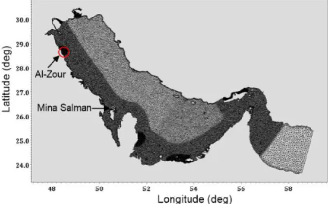
Al-Zour has become a major industrial complex, in which many power plants and oil refinery plants have been constructed and operated. The Al-Zour LNG import terminal project and the expansion planning of an existing power plant are also in progress (Fig. 1). The LNG supplied by the facility is expected to feed power plants in Kuwait, enabling them to generate enough power to meet electricity demand during peak times.
In Kuwait, industrial plants have been developed in clusters in specific complexes supporting common infrastructures and utilities.
Therefore, the sea-water intakes and outfall facilities of additional projects tend to be installed adjacent to those of existing plants, which make the prediction of local seawater temperature change
* First Author : [email protected], 02-746-0163
†Corresponding Author : [email protected], 061-240-7319
around the construction site more complicated due to thermal discharge from neighboring plants. For the LNG import terminal project, the location is only 3 kilometers north of a power plant where massive thermal and brine water is being discharged.
Therefore, the supply of water for the LNG re-gasification facility is expected to be influenced by the thermal discharge of such power plants.
It is important to assess the seawater temperature accurately and predict future seawater temperature change according to possible expansion plans. Many researchers have modeled the hydrodynamic in the Arabian Gulf (e.g., John, 1992; Chao et al., 1992;
Hosseinibalam et al., 2011; Pous et al., 2012; Ganj, 2013), but smaller-scale numerical simulation is required to account for the influence of adjacent thermal discharge at a specific site.
In this study, the seawater temperature variations around the Al-Zour LNG import terminal are investigated through MIKE 3 numerical modeling. The model is capable of simulating current dynamics and temperature variations simultaneously. Most of meteorological input in the numerical simulation was obtained from the European Re-Analysis (ERA) hindcast data provided by the European Centre for Medium Range Weather Forecasts (ECMWF).
The ERA-interim and ERA-5 data from ECMWF is open-accessible and free to download for all uses, including for commercial use. A
Numerical Simulation of the Water Temperature in the Al-Zour Area of Kuwait
Myung Eun Lee
*․ Gunwoo Kim
**†* R&D Center, Hyundai Engineering & Construction Co., 75 Yolgok-ro, Seoul 03058, Republic of Korea
** Department of Ocean Civil Engineering, Mokpo National Maritime University, 91 Haeyangdaehang-Ro, Mokpo 58628, Republic of Korea
Abstract :The Al-Zour coastal area, located in southern Kuwait, is a region of concentrated industrial water use, seawater intake, and the outfall of existing power plants. The Al-Zour LNG import facility project is ongoing and there are two issues regarding the seawater temperature in this area that must be considered: variations in water temperature under local meteorology and an increase in water temperature due to the expansion of the thermal discharge of expanded power plant. MIKE 3 model was applied to simulate the water temperature from June to July, based on re-analysis data from the European Centre for Medium-Range Weather Forecasts (ECMWF) and the thermal discharge input from adjacent power plants. The annual water temperatures of two candidate locations of the seawater intake for the Al-Zour LNG re-gasification facility were measured in 2017 and compared to the numerical results. It was determined that the daily seawater temperature is mainly affected by thermal plume dispersion oscillating with the phase of the tidal currents. The regional meteorological conditions such as air temperature and tidal currents, also contributed a great deal to the prediction of seawater temperature.
Key Words :Kuwait, MIKE3, Numerical simulation, Thermal discharge, Water temperature
first segment of the data set (ERA-interim) is now available for public use (from 1979 to within three months of present time) and provides six hourly estimates for spatial resolution of 0.7° of a large number of atmospheric, land and oceanic climate variables.
Calibrations of the model are carried out against the re-analysis data of the ECMWF. The established model is applied to the prediction of water temperature considering the thermal discharge from the southern power plant. The simulated water temperature is compared to in-situ water temperature measurement.
Fig. 1. Location of the Al-Zour LNG import terminal and seawater temperature monitoring points (from Google Map).
2. Hydrodynamic Model
2.1 MIKE 3-FM model
The hydrodynamic and thermal simulation of the Al-Zour site was conducted using MIKE 3-FM (Flexible Mesh) of DHI. The modelling system is based on the numerical solution of three-dimensional incompressible Reynolds-averaged Navier-Stokes equations subject to the assumptions of Boussinesq and hydrostatic pressure. Thus, the model consists of continuity, momentum, temperature, salinity and density equations and is closed by a turbulent closure scheme. The free surface is taken into account using a sigma-coordinate transformation approach.
The local continuity equation is written as
(1)
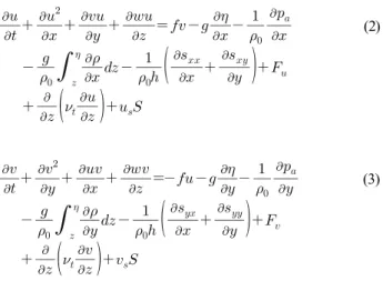
and the two horizontal momentum equations for the - and - components, respectively, are written as
(2)
(3)
where is the time; , and are the Cartesian coordinates; is the surface elevation; , and are the velocity components in the , and direction; sin is the Coriolis parameter ( is the angular rate of revolution and the geographic latitude); is the gravitational acceleration; is the density of water; and are components of the radiation stress tensor; is the vertical turbulent (or eddy) viscosity; is the atmospheric pressure; is the reference density of water. is the magnitude of the discharge due to point sources and is the velocity by which the water is discharged into the ambient water. The horizontal stress terms are described using a gradient-stress relation, which is simplified to
(4)
(5)where is the horizontal eddy viscosity.
The fluid is assumed to be incompressible. Hence, the density,
, does not depend on pressure, but only on temperature, , and the salinity, via the equation of state
(6)
The transports of temperature, , and salinity, , follow the general transport-diffusion equations as
(7)
(8)
where is the vertical turbulent diffusion coefficient. is a source term due to heat exchange with the atmosphere. and are the temperature and the salinity of the source. are the horizontal diffusion terms defined by
(9)where is the horizontal diffusion coefficient.
MIKE 3 simplifies the vertical momentum equation by the assumption of Boussinesq, which is generally valid for the continental shelf where the bottom topography is mild. This model can also reproduce the passive thermal transport and dispersion properly, considering the open channel discharge of thermal effluent.
2.2 Climate characteristics
Al-Zour area has a long, dry, hot summer, with temperatures often reaching 50℃ while air temperature may fall to 0℃ in winter (Al-Yamani et al., 2004). Seawater temperature is highest in August and lowest in January. Uddin et al. (2011) reported that the measured seawater temperature during 1991 and 2003 by the Kuwait Environment Public Authority (KEPA) at the Ras Al-Zour station showed a maximum value of 35℃ in summer and a minimum value of 14℃ in winter. Pokavanich et al. (2015) also provided the measured seawater temperature at off-Khiran (20°56.805′N, 48°34.397′E). The data ranged from 15℃ to 3 5℃ for the year, which is very similar to the measured temperature by Uddin et al. (2011). The ECMWF ERA-interim
reanalysis climatology data at 28.66°N, 48.43°E indicated that the annual mean seawater temperature wa 25.03℃ from 1979 to 2015.
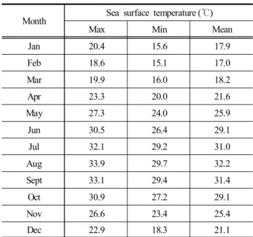
The maximum and minimum seawater temperature was 33.9℃ in August and 15.1℃ in February, respectively. Table 1 shows the monthly maximum, minimum and mean values of seawater temperature at Al-Zour area, obtained from the ERA-interim reanalysis data.
Month Sea surface temperature (℃)
Max Min Mean
Jan 20.4 15.6 17.9
Feb 18.6 15.1 17.0
Mar 19.9 16.0 18.2
Apr 23.3 20.0 21.6
May 27.3 24.0 25.9
Jun 30.5 26.4 29.1
Jul 32.1 29.2 31.0
Aug 33.9 29.7 32.2
Sept 33.1 29.4 31.4
Oct 30.9 27.2 29.1
Nov 26.6 23.4 25.4
Dec 22.9 18.3 21.1
Table 1. Seawater temperatures near the Al-Zour Location during 1979-2015 (ECMWF ERA-interim model)
We measured the water temperature at two candidate locations (T1 and T2 in Fig. 1) for the LNG terminal facility in five- minute intervals from February to December 2017. The coordinates of T1 and T2 and the water depth of measurement at each location are described in Table 2.
Measurement Location T1 T2
Water depth (m) 10.5 8.5
Coordinates Latitude (N) 28°43′47.9″ 28°43′15.1″
Longitude (E) 48°24′34.7″ 48°24′27.2″
Measurement depth (m)
Surface 5.5 3.4
Middle 7.7 5.5
Bottom 10.0 7.7
Table 2. Coordinates and water depth of measurement at T1 and T2
2.3 Model setup
We used the Mike 3 model, which is a general numerical modeling system for the simulation of flows in estuaries, bays and coastal areas as well as in oceans. The model grid was nested from the Arabian Gulf regional tidal model to provide open-boundary conditions on the nested boundaries. The regional model covers the entire Arabian Gulf and part of Oman. Fig. 2 shows the regional model domain and mesh distribution. The resolution of mesh ranges from 800 to 12000 meters. Along the open boundary, FES2012 (Le Provost et al., 1998; Carrere et al., 2012) was used as open boundary condition. On the surface, the model was forced by the atmospheric pressure and wind fields derived from the ECMWF data set. Fig. 3 shows the comparison between the simulated and measured water level at Mina Sulman in Bahrain, which was collected from the Sea Level Center of University of Hawaii (http://uhslc.soest.hawaii.edu/data/?rq).
Fig. 2. Mesh distribution in regional model domain.
Fig. 3. Comparison between simulated and measured water level at Mina Salman in Bahrain.
The nested Al-Zour model was developed in 5-sigma vertical layered model with 14,173 elements of horizontal triangular grid.
The minimum size of the mesh is 20 meters around the power plant outfalls, and maximum size is 1 kilometer near the open boundaries. The bathymetry was obtained from the MIKE C-MAP digital chart. The nested model covers 20 kilometers towards the shoreline and 35 kilometers of an along-shore line. Fig. 4 shows the project area and nearby facilities.
The Smagorinsky (1963) formulation was applied for the horizontal eddy viscosity with a calibrated coefficient of 0.28 from the regional model. For the vertical turbulence model, MIKE 3 used k- formulation with the recommended empirical constants by Rodi (1980). Bottom resistance was set by the roughness height with a constant value 0.05 meters considering the mean diameters (0.003 ~ 0.19 m) at the northwestern part of the Arabian Gulf (Khaleghi et al., 2014).
Fig. 4. Al-Zour hydrodynamic model mesh including nearby facilities.
In order to consider the seawater temperature variations, the baroclinic module with a density considered to be a function of the temperature was selected. The heat exchange with the atmosphere
was calculated on the basis of four physical processes: latent heat flux, sensible heat flux, net short-wave radiation, and net long-wave radiation. For the calculation of latent heat, the default coefficients of MIKE 3 were used, as recommended in DHI (2016). For the calculation of sensible heat exchange, a heating coefficient of 0.0011 and cooling coefficient of 0.008 were used, following the recommended default value of DHI (2016). The atmospheric temperature input for the sensible heat was chosen from two sources: the ECMWF hindcast reanalysis data ERA-interim and the hourly records of meteorological observation in Kuwait City. The time varying net short-wave radiation was included from the extracted data of the ERA-interim data set of the ECMWF. The maximum surface short-wave radiation reached 978 W/m2 from June to July in 2017 in this area. The long-wave radiation between the water surface and the atmosphere was also included by Brunt’s equation which is implemented in the MIKE 3 model using the same air temperature input for sensible heat calculation.
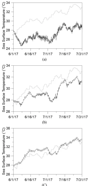
Relative humidity and clearance were set as 17 % and 70 %, respectively, for the whole simulation period. The seawater temperature along the open boundary was obtained from the surface water temperature in six hourly data of the ERA-interim data set (see Fig. 5). The numerical simulation was conducted from June to July in 2017 and compared to the measured or re-analyzed water temperatures.
Fig. 5. Sea surface temperature for boundary condition extracted from ERA-interim data set.
3. Numerical Simulation
3.1 Model calibration
Model calibration was carried out at T1 location with the sea surface temperature obtained from the ERA-interim data set, which
does not include influence by local thermal discharge from the southern power plant due to its coarse grid. Therefore, the calibration of various parameters in the model was made possible by modeling only with meteorological conditions such as air temperature, short-wave radiation and wind speed etc. In this sense, natural heat transfer in the water body was described without interruption of the thermal discharge.
(a)
(b)
(C)
Fig. 6. Comparison of heat exchange with various parameter settings: dashed line = ERA-interim water temperature, solid line = numerical result at T1 surface, (a) open boundary input + air temperature from ERA-interim data (b) including short wave radiation (c) substituting the measured air temperature at Kuwait City as input data.
Fig. 6 shows a comparison of surface water temperature variations between the ERA-interim data and the simulated sea surface temperature in regard to only the sea surface water temperature when the open boundary conditions and air temperature are implemented (sequence a), when the short and long-wave radiation effects are included (sequence b), and when the measured air temperature in Kuwait City is used for input data instead of the air temperature from ERA-interim data set (sequence c). All the sequences showed that the wave radiation and the use of measured air temperature improved the accuracy of the prediction of water temperature. Table 3 shows the root mean square error (RMSE) and normalized root mean square error (NRMSE) for each sequence.
Sequences RMSE(℃) NRMSE(%)
(a) 3.95 78.5
(b) 1.76 34.0
(c) 0.80 13.6
Table 3. Comparison of calibration results
3.2 Simulation with thermal discharge
In this section, the influence of the thermal discharge from adjacent power plants was assessed. Local hydrodynamics during the simulation period was reproduced by including the thermal discharge from the southern power plant. Thermal discharge from the surface outfall of the southern power plant was considered as 131 m3/s of flowrate and 6℃ of excess water temperature in the one-through cooling system. It should be noted that the information of thermal discharge is roughly averaged values because a detailed operational record of the power plant was not available.
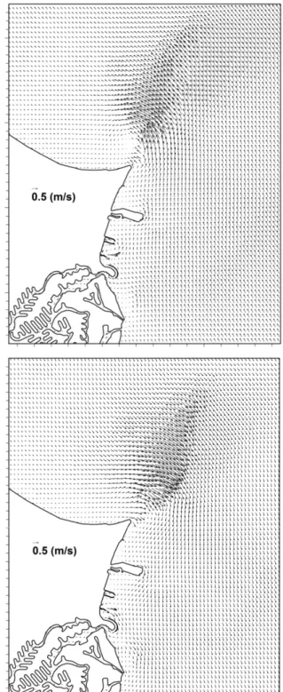
Fig. 7 shows the tidal current patterns for the flood (a) and ebb (b) tides. The mean current speed around the site ranges between 0.1 m/s and 0.15 m/s, whereas it reaches 0.4 m/s at the Al-Zour reef area in the northern part of Kuwait LNG import site. the maximum current speed around the site is 0.2 m/s to 0.3 m/s, while the current speed at the Al-Zour coral reef area reaches 0.7 m/s.
Fig. 8 shows the seawater temperature distribution for the flood and ebb tide. Discharged plume from the southern power plant outfall moved back and forth in north-and-south direction, forming a large thermal cloud from the entrance of the Al Khiran resort to the corner of the coral reef area. Most of the discharged thermal plumes were blocked by the LNG facility which was formed by
land reclamation work. However, for flood tides, a portion of the thermal plumes went over the LNG facility, which increased the water temperature at T1 and T2. For the ebb tide, the water temperature at T1 and T2 were not highly influenced by the thermal discharge.
Fig. 7. Local hydrodynamics for flood (left) and ebb (right) tide.
(a) Flood tide
(a) Ebb tide
Fig. 8. Sea surface water temperature distribution with thermal discharge from power plant for flood and ebb tide.
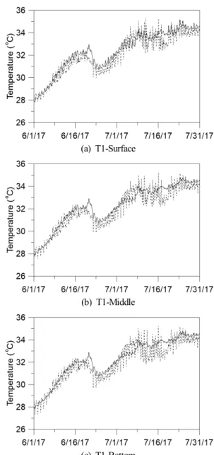
The overall rise of measured water temperatures during the simulation period was compared with simulation results at each location in Fig. 9 and 10. The results showed a good agreement with the daily mean temperature increase in measurement, especially at the surface measurement point. Temperature
fluctuation peaks occurred when the sea current direction was running north, i.e. the flood tide. The amplitude of fluctuations were higher in the measured temperature than in the simulation results.
(a) T1-Surface
(b) T1-Middle
(c) T1-Bottom
Fig. 9. Comparison between simulated and measured temperature at T1: dashed line = measured data, solid line = numerical simulation.
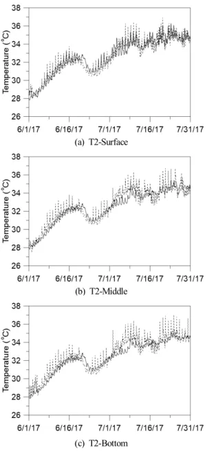
The water temperature at T2 was more dependent on the dispersion of thermal discharge from the power plant than the temperature at T1 because T2 is closer to the outfall of power plant. Fluctuations in the simulation results reach approximately 2℃ and 1℃ for T2 and T1, respectively. This amplification is two
to four times larger than the 0.5℃ fluctuation of thermal plume temperature in the calibration without thermal discharge (Fig. 10).
(a) T2-Surface
(b) T2-Middle
(c) T2-Bottom
Fig. 10. Comparison between simulated and measured temperature at T2: dashed line = measured data, solid line = numerical simulation.
Measurement(℃) Simulation(℃)
T1 T2 T1 T2
Surface 35.34 36.91 35.15 36.29
Middle 35.25 36.72 34.76 35.40
Bottom 35.23 37.03 34.72 35.14
Table 4. Comparison of maximum water temperature.
The maximum temperature of the measurement and simulation results are listed in Table 4. The maximum surface water temperatures at T1 and T2 were, respectively, recorded as 35.34℃
and 36.91℃, which implies that the thermal discharge from the power plant increased the local water temperature 1.7℃ and 3.3℃
for T1 and T2, respectively, compared to the ERA-interim data.
The simulated results underestimated the maximum temperature 0.2~0.6℃ at surface layer. Especially, at the bottom layer, the temperature underestimation becomes 0.5~1.9℃. Table 4 shows that there is a little temperature difference between the surface layer and bottom layer.
(a) Surface
(b) bottom
Fig. 11. Comparison of measured and simulated water temperature: circle at T1, filled circle at T2.
Comparisons of the measured and simulated water temperatures at the surface and bottom layers of T1 and T2 are shown in Fig.
11. The results at the surface layer show better agreement than those at the bottom. For the bottom layer, the results at T1 show slightly better agreement than those at T2. At the surface layer, correlation coefficients were calculated as 0.962 and 0.955, respectively, for T1 and T2, while at the bottom, correlation coefficients were 0.948 and 0.944. Although the overall agreement is acceptable at the bottom layer, the simulation overestimated at T1 for the ebb tide and underestimated at T2 for the flood tide.
Considering normal thermal stratification of discharged water on the surface, the weak vertical stratification in measurement shows that there exists strong vertical mixing due to the strong discharge momentum.
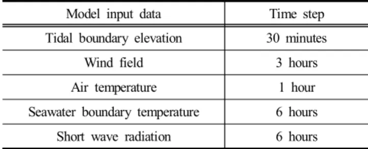
It should be noted that seawater temperatures at T1 and T2 were measured every five minutes, whereas the intervals of model input data were much longer than that of measurement as in Table 5.
Three hourly averaged wind fields and one hourly averaged air temperature were not sufficient to consider a gust reproducing the temporal peak current and a fluctuation in heat exchange between air and sea surface. In addition, the use of a relatively coarse grid may also be a cause of the numerical diffusion. The numerical simulation will be able to reproduce measured data more accurately if the detailed thermal outfall operation record is provided as input data.
Model input data Time step
Tidal boundary elevation 30 minutes
Wind field 3 hours
Air temperature 1 hour
Seawater boundary temperature 6 hours
Short wave radiation 6 hours
Table 5. Time steps of input data.
4. Conclusions
In this study, the sea water temperature around the Al-Zour LNG import terminal was investigated by using MIKE 3 numerical model with the thermal discharge from an adjacent power plant.
The model was calibrated by wave radiation and air temperature.
The simulated water temperatures were compared to in-situ water temperature measurement. The simulation results showed a good agreement with the daily mean temperature increase in the
measurement on the surface layer, but the simulated results underestimated the maximum temperature by 0.5~1.9℃ at the bottom layer. It was found that the sea water temperature variation in this area is greatly affected by the local thermal plume dispersion oscillating with the phase of the tidal current.
References
[1] Al-Yamani F., B. James, R. Essa, M. Al-Husaini and A.
Al-Ghadan(2004), Oceanographic atlas of Kuwait’s waters, KISR publication, Kuwait, pp. 81-191.
[2] Carrere, L., F. Lyard, M. Cancet, A. Guillot and L.
Roblou(2012), FES2012: A new tidal model taking advantage of nearly 20 years of altimetry measurements, Proc. 20 Yrs.
Prog. in Rad. Alt. Symp. ESA SP-710, CD-ROM.
[3] Chao, S. Y., T. W. Kao, and K. R. Al-Hajri(1992), A Numerical investigation of circulation in the Arabian Gulf, J.
Geophys. Res., Vol. 97, pp. 11219-11236.
[4] DHI(2016), MIKE 21 & MIKE 3 Flow Model FM Hydrodynamic Module Scientific Documentation.
[5] Ganj, M.(2013), Simulation of tidal currents in the Persian Gulf, Int. J. Emerg. Trends Eng. Dev., Vol. 5, pp. 31-38.
[6] Hosseinibalam, F., S. Hassanzadeh and A. Rezaei-Latifi(2011), Three-dimensional numerical modeling of thermohaline and wind-driven circulations in the Persian Gulf, Appl. Math.
Model., Vol. 35, pp. 5884-5902.
[7] John, V. C.(1992), Harmonic tidal current constituents of the western Arabian Gulf from moored current measurements, Coast. Eng. Vol. 17, pp. 145-151.
[8] Khaleghi, A., M. Soltanpour and S. A. Haghshenas(2014), A study on the sand-mud mixture at north-western part of the Persian Gulf, Int. Conf. Coast. Eng., Vol. 1(34), DOI:
https://doi.org/10.9753/icce.v34.sediment.79.
[9] Le Provost, C., F. Lyard, J. M. Molilnes, M. L. Genco and F.
Rabilloud(1998), A hydrodynamic ocean tide model improved by assimilating a satellite altimeter-derived data set, J.
Geophys. Res., Vol. 103, pp. 5513-5529.
[10] Pokavanich, T., Y. Alosairi, R. Graaff, R. Morelissen, W.
Verbruggen, K. Al-Refail, A. Taqi and T. Al-Said(2015), Three-dimensional Arabian Gulf hydro- environmental modeling using DELFT 3D, E-proc. of the 36th IAHR World Cong.
[11] Pous, S., X. Carton and P. Lazure(2012), A process study of the tidal circulation in the Persian Gulf, Open J. Mar. Sci., Vol. 2, No. 4, pp. 131-140.
[12] Rodi, W.(1980), Turbulence Models and Their Application in Hydraulics - a State of the Art Review, Special IAHR Publication.
[13] Smagorinsky, J.(1963), General circulation experiments with the primitive equations: 1. The basic experiment. Monthly Weather Review, Vol. 91, No. 3, pp. 99-164.
[14] Uddin, S., A. N. Al Ghadban and A. Khabbaz(2011), Localized hyper saline waters in Arabian Gulf from desalination activity, Env. Mon. Assess, Vol. 181, pp. 587-594.
Received : 2019. 05. 10.
Revised : 2019. 05. 27.
Accepted : 2019. 05. 28.