LBCC of Transient State for High Strength Steel in Hot Strip Mills

(1)

DOI:10.5302/J.ICROS.2011.17.4.382 ISSN:1976-5622 eISSN:2233-4335

I.

서론

.

1000MPa ,

. ,

ROT (Run-Out Table) . ROT , (roughing mill), (finishing mill)

(phase transformation) [1].

ROT

.

(head part) (tail part) [2,3].

. ,

, (header) (quantity of cooling water) .

. ,

, .

,

* (Corresponding Author)

: 2010. 11. 30., : 2011. 1. 14., : 2011. 1. 17.

, :

([email protected]/[email protected])

2009 .

(loop)

. ,

.

(center) (edge)

.

, .

. ROT

. ROT ,

, .

,

ROT [4,5].

(bank) [6].

[7,8].

(history)

[9,10]. ROT (heat flux)

[11-13]. ,

, ,

[14,15].

LBCC

LBCC of Transient State for High Strength Steel in Hot Strip Mills

*,

(Cheol Jae Park

¹

and Kang Sup Yoon

¹

)

1Daegu University

Abstract: In this paper, a LBCC (Latter Bank Cooling Control) for the high strength steel is proposed to obtain the desirable

temperature and the property of the material along the longitudinal direction of the steel on the ROT (Run-Out Table) process.

A cooling valve is modeled to analyze the response of the ROT banks. The control concept is derived from a field data, a valve model considering the valve response and a TTT (Time-Temperature Transformation) diagram. The proposed control is verified from the simulation results under the various carbon quantities. It is shown through the field test of the hot strip mill that the deviation of the CT (Coiling Temperature) is considerably decreased by the proposed temperature control.

Keywords: hot strip mills, temperature control, latter bank, bank response, valve model, high strength steel

(2)

ROT

(LBCC: Latter Bank Cooling Control) .

.

LBCC .

,

ROT .

, .

프로세스와 온도제어 문제

II. ROT

프로세스 1. ROT

1 ROT

. ROT 16 (#1~#16)

, / (control valve)

. ROT FDT (Finishing Delivery Temperature), MT (Middle Temperature), CT (Coiling Temperature) 3

.

ROT (FDT),

, ,

. 1~14

6 . CT

15~16 12

. ROT

4 , ,

, , .

ROT

. FDT

. ,

.

고강도강의 온도제어 문제점 2.

ROT ,

(step) . 2

.

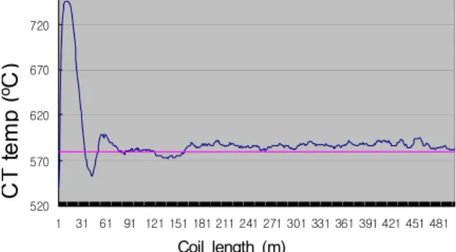
. , CT

600

^o

C , 40m

670

^o

C, 30m 650

^o

C

. ,

. 3

.

580

^o

C 200

^o

C .

.

4 TTT

(time-temperature transformation) . FDT

ROT 4

1. ROT .

Fig. 1. Configuration of ROT in hot strip mills.

2. .

Fig. 2. Step cooling pattern of hot strip steel.

CT temp (o C)

520 570 620 670 720

1 31 61 91 121 151 181 211 241 271 301 331 361 391 421 451 481

Coil length (m)

3. .

Fig. 3. Temperature deviation by step cooling in head part.

(3)

(bainite)

, 100%

.

(pearlite) 4 .

, .

.

뱅크 응답성을 고려한 알고리즘 개발

III. LBCC

냉각뱅크의 응답성을 고려한 밸브 모델링 1.

(LBCC) . ROT

, .

.

. ,

0.8 1.2 .

1 .

5. .

Fig. 5. Valve response for step input (T

r

=1sec).



_{  }

 







(1)

T

63.2%

, K .

90%

(T

r

) ,

1.2 1 .

(1)

T

0.45, K 1

, 5

.

뱅크 응답성을 고려한 알고리즘 개발

2. LBCC

LBCC

(backward)

.

FDT ,

. 6

ROT FDT 14

y14

z14

14 .

V mpm

, (1)

14 .



_

  

_

  





×  (2)

  







^{ }^



(3)

_{}

_{  }



_



_

× 

_

 

_

 (4)

x14

(t): 14 (m)

y14

: FDT 14 (m)

z14

: 14

V(t):

(mpm)

Pbc,14

(t): 14

Pearlite 변태곡선(1%)

Bainite 변태곡선(1%) 50%

100%

100%50%

FDT 온도

4. TTT .

Fig. 4. TTT diagram of high strength steel.

(4)

6. LBCC . Fig. 6. Bank layout of LBCC algorithm.

7. LBCC .

Fig. 7. Basic concept of LBCC algorithm.

7 LBCC

. '1P', '2P' 1 , 2

, FDT

.

14 , 13

. LBCC .

Step 1: (1)

Pbc,14

(4) ,

FDT 14 .

Step 2: 14 ,

1~13 . , 14

, 1~13 CT

CT . , CT

.

_{}



_

 



₍₅₎

CTt,adj

CT , CT

t

CT

,

ΔCT

14 .

Step 3:

Pbc,14

2~3

CT

CT .

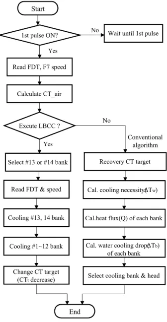
8 LBCC

.

1st pulse ON?

Yes

Read FDT, F7 speed

Start

Calculate CT_air

Excute LBCC ?

Cooling #13, 14 bank

Cooling #1~12 bank

Cal. cooling necessity( ∆T

w

)

Cal.heat flux(Q) of each bank Select #13 or #14 bank

Conventional algorithm

End

No

Yes

Read FDT & speed

Cal. water cooling drop( ∆T

b

) of each bank

Wait until 1st pulse No

Select cooling bank & head Change CT target

(CT

t

decrease)

Recovery CT target

8. LBCC .

Fig. 8. Flowchart of LBCC algorithm.

시뮬레이션을 통한 알고리즘 검증 3.

LBCC ,

. .

.

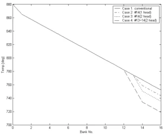
9 2.3mm

.

1 .

(5)

. .

LBCC .

CT

752

^o

C .

1~13

14 1

CT 743.6

^o

C . 1~13

, 14 .

(15, 16 ) 15~16

. 2

8.4

^o

C .

14 2

. CT

735.1

^o

C .

,

4 16.9

^o

C

.

13 14 2

CT 718.8

^o

C

. 8

33.2

^o

C .

,

. 온라인 테스트 결과

IV.

.

10 LBCC

. CT

, CT

. 2.0mm, (

0.85%) , CT 620

^o

C .

CT ( CT CT ) .

13, 14

2 .

600

^o

C

. 4 TTT

,

.

. LBCC

CT ,

75

^o

C 38

^o

C ,

11.7

^o

C 5.5

^o

C 52.9% .

11 0.45% 2.0mm,

CT 640

^o

C .

9. LBCC .

Fig. 9. Simulation result of LBCC algorithm.

1. LBCC .

Table 1. Simulation condition of LBCC.

Parameter Value Parameter Value

(mm) 2.3 CT(

^o

C) 540

(mm) 1000 (mpm) 640

FDT(

^o

C) 880 (W/m

^{2 o}

C) 1.0

10. (C: 0.85%, CT: 620

^o

C).

Fig. 10. On-line test result(C: 0.85%, CT: 620

^o

C).

11. (C: 0.45%, CT: 640

^o

C).

Fig. 11. On-line test result(C: 0.45%, CT: 640

^o

C).

(6)

CT , 55

^o

C

5

^o

C , 5.8

^o

C 3.4

^o

C 41.4%

.

V.

결론 ROT

,

(LBCC) ,

, .

,

.

,

CT

41% ,

.

참고문헌

[1] N. S. Samaras and M. A. Simaan, “Optimized trajectory tracking control of multistage dynamic metal-cooling processes,” IEEE Transactions on Industry Applications, vol. 37, no. 3, pp. 920-927, 2001.

[2] A. G. Groch, R. Gubernat, and E. R. Birstein,

“Automatic control of laminar flow cooling in continuous and reversing hot strip mills,” Iron and Steel

Engineer, vol. 67, no. 9, pp. 16-20, 1990.

[3] S. K. Biswas, S. Chen, and A. Satyanarayana, “Optimal temperature tracking for accelerated cooling processes in hot rolling of steel,” Dynamics and Control, vol. 7, pp.

327-340, 1997.

[4] R. K. Kumar, S. K. Sinha, and A. K. Lahiri, “An on-line parallel controller for the runout table of hot strip mills,” IEEE Transactions on Control Systems

Technology, vol. 9, no. 6, pp. 821-830, 2001.

[5] S. Guan, H. X. Li, and S. K. Tso, “Multivariable fuzzy supervisory control for the laminar cooling process of hot rolled slab,” IEEE Transactions on Control Systems

Technology, vol. 9, no. 2, pp. 348-356, 2001.

[6] G. V. Ditzhuijzen, “The controlled cooling of hot rolled strip: a combination of physical modeling, control problems and practical adaptation,” IEEE Trans. on

Automatic Control, vol. 38, no. 7, pp. 1060-1065, 1993.

[7] M. D. Leltholf and J. R. Dahm, “Model reference

control of runout table cooling at LTV,” Iron and Steel

Eng., vol. 66, no. 8, pp. 31-35, 1989.

[8] N. S. Samaras and M. A. Simaan, “Water-cooled end-point boundary temperature control of hot strip via dynamic programming,” IEEE Transactions on Industry

Applications, vol. 34, no. 6, pp. 1335-1341, 1998.

[9] F. E. James et al., “Numerical modeling of hot strip mill runout table cooling,” Iron Steel Eng., pp. 50-55, 1993.

[10] N. Hatta and H. Osakabe, “Numerical modeling for cooling process of a moving hot plate by a laminar water curtain,” The Iron and Steel Institute of Japan, vol. 29, no. 11, pp. 919-925, 1989.

[11] W. Timm, K. Weinzierl, A. Leipertz, H. Zieger, and G.

Zouhar, “Modelling of heat transfer in hot strip mill runout table cooling,” Steel Res., vol. 73, no.3, pp.

97-104, 2002.

[12] T. Oda, Y. Kondo, S. Konishi, H. Murakami, M.

Suehiro, and T. Yabuta, “Development of accurate control in hot strip mill,” The Iron and Steel Institute of

Japan, vol. 81, no. 3, pp. 35-40, 1995.

[13] N. S. Samaras, “Novel control structure for runout table coiling temperature control,” AISE Steel Tech., 2001.

[14] D. Auzinger and F. Parzer, “Process optimization for laminar cooling,” MPT International, vol. 5, pp. 68-75, 1996.

[15] E. N. Hinrichsen and G. P. Petrus, “Hot strip mill runout table cooling: a system view of control, operation and equipment,” Iron and Steel Eng., vol. 53, no. 10, pp. 29-34, 1976.

박 철 재 1992

( ). 1994 (

). 2008

( ). 1994 ~2008 . 2008 9

~

. , ,

, .

윤 강 섭 1986

( ). 1988

( ). 1997

~2000

. 2000 ~

. , ,

ITS .