J. Korean Soc. of Marine Engineering (JKOSME) ISSN 2234-8352 (Online)
http://dx.doi.org/10.5916/jkosme.2016.40.5.389 Original Paper
This is an Open Access article distributed under the terms of the Creative Commons Attribution Non-Commercial License (http://creativecommons.org/licenses/by-nc/3.0), which permits unrestricted non-commercial use, distribution, and reproduction in any medium, provided the original work is properly cited.
†Corresponding Author (ORCID: http://orcid.org/0000-0002-6221-822x): Department of Energy and Mechanical Engineering, Gyeognsang National University, E-mail: [email protected], Tel: 055-772-9110
1 Devision of Marine System Engineering, Korea Matitime and Ocean University, E-mail: [email protected], Tel: 051-410-4257 2 Devision of Marine System Engineering, Korea Matitime and Ocean University, E-mail: [email protected], Tel: 051-410-4228 3 Offshore Commissioning Team, Daewoo Shipbuilding & Marine Engineering, E-mail: [email protected], Tel: 055-735-2114
Analytical solution of the Cattaneo Vernotte equation (non-Fourier heat conduction)
Jae Hyuk Choi1 ․ Seok-Hun Yoon2 ․ Seung Gyu Park3 ․ Soon-Ho Choi† (Received February 29, 2016; Revised March 21, 2016;Accepted May 2, 2016)
Abstract: The theory of Fourier heat conduction predicts accurately the temperature profiles of a system in a non-equilibrium steady state. However, in the case of transient states at the nanoscale, its applicability is significantly limited. The limitation of the classical Fourier’s theory was overcome by C. Cattaneo and P. Vernotte who developed the theory of non-Fourier heat con- duction in 1958. Although this new theory has been used in various thermal science areas, it requires considerable mathemat- ical skills for calculating analytical solutions. The aim of this study was the identification of a newer and a simpler type of solution for the hyperbolic partial differential equations of the non-Fourier heat conduction. This constitutes the first trial in a series of planned studies. By inspecting each term included in the proposed solution, the theoretical feasibility of the solution was achieved. The new analytical solution for the non-Fourier heat conduction is a simple exponential function that is com- pared to the existing data for justification. Although the proposed solution partially satisfies the Cattaneo–Vernotte equation, it cannot simulate a thermal wave behavior. However, the results of this study indicate that it is possible to obtain the theoretical solution of the Cattaneo–Vernotte equation by improving the form of the proposed solution.
Keywords: Cattaneo–Vernotte equation, Hyperbolic type partial differential equation, Non-Fourier heat conduction
1. Introduction
A heat wave, also known as a thermal wave, constitutes a subject of intense research but it is still an ambiguous concept in thermal science and engineering. At present, the phenomena elicited by a thermal wave are being applied to nondestructive examinations (NDE) [1] or skin care applications [2]. These applications utilize the physical characteristics of materials giv- en that the thermal conductance and the thermal relaxation times are different in a variety of materials. Thermal con- ductance is the rate of heat absorption and thermal relaxation is the rate of heat dissipation.
The concept of non-Fourier heat conduction resulted from the newly issued heat conduction mechanism that modified Fourier’s heat conduction theory, which was issued by C.
Cattaneo and P. Vernotte independently in 1958 [3]. The de- fect of the Fourier heat conduction equation was originally in- dicated by J. C. Maxwell in 1867 with the comment that it implies the use of an infinite propagation speed for a thermal disturbance in a medium [4].
The heat conduction phenomena in solids are well predicted
by the classical Fourier heat conduction equation in almost all engineering cases. Nevertheless, it cannot be applied to specif- ic scientific cases that deviate from the conventional ones, which usually include the heat transfer phenomena at the nanoscale, periodic heat fluxes, laser heating, or the presence of a cryogenic region [5]. According to recent studies, the wave characteristics appear in a heat transfer process under some specialized conditions or applications.
The term “wave” implies that some physical quantities pos- sess specific characteristics, such as the wavefront, and its re- flection or refraction at a boundary. Additionally, if a heat transfer phenomenon can be treated by the wave theory, matter should possess the dual properties of wave and particle simul- taneously as heat transfer in solids can be interpreted by an imaginary particle known as the phonon that possesses wave- like properties [6].
On the other hand, some studies argue that the concept of a thermal wave was not valid because there are no ob- servations of the wavelike characteristics, and because an ap- plied thermal transient does not travel fast in a medium as a wave does, but rather diffuses in it [7]. However, this study
is not concerned on whether a thermal disturbance is wave- like (or not) since the purpose herein is to find the simple type of the mathematical solution for the governing equation of a thermal wave.
Based on the investigations by the authors in prior studies on thermal waves [8][9], a thermal disturbance in any material is expected to be propagated with an infinite velocity. In the real world, the infinite propagation speed of a thermal wave is not possible although it can be assumed to be reasonable un- der specific, constrained conditions.
According to the study of Marvin Chest [10], the square of the thermal wave velocity (CT) is one third of the square of the phonon velocity (CA), that is CT2
= CA2
/3. The thermal wave, which is the main feature of non-Fourier heat con- duction, became after this initial study the focus of research work relevant to thermal phenomena.
Specifically, in reference to typical studies on the non-Fourier heat conduction, J. Gembarovic et al. [11] pre- sented an analytical solution for heat pulse propagation in a one- dimensional system using the Dirac-delta function, the Heaviside unit step function, the Laplace transform, and the Inverse transform. D. D. Joseph et al. [3] derived the govern- ing equations and introduced the procedures to calculate the temperature field and the heat flux in a system. However, he did indicate that Fourier’s heat conduction equation has still practical authority in science and engineering because the ther- mal relaxation time is extremely short compared to the time scale of events in our daily lives, which is the distinctive dif- ference between the Fourier and non-Fourier heat conductions.
K. K. Tamma et al. [4] published a study on the thermal transport phenomena at macroscale and microscale systems.
More recently, significant additional attention has been paid on non-Fourier heat conduction due to its potential applications to the fields of laser heating processes [12] and microscale heat transfer [13]. C. W. Chang et al. indicated that the prediction of heat conduction based on Fourier’s heat conduction theory largely deviated from the experimental data when a system had a low dimension (for example, one dimension, such as the case of a carbon nanotube or a chain) [14].
Megan Jaunich et al. performed an experiment to investigate the temperature distribution when a laser beam irradiated the skin tissue [15]. According to their findings, the experimental results disagreed with the predictions of Fourier’s heat con- duction equation but agreed with the calculated results based on the non-Fourier’s heat conduction equation.
As mentioned previously, despite the fact that so many ther- mal scientists have concentrated their efforts on non-Fourier heat conduction phenomena, it is somewhat difficult to com-
prehend the theory thoroughly. To understand it, elaborate mathematical skills are required.
Accordance to the authors’ viewpoints, the previous ana- lytical studies require a profound mathematical knowledge to understand the non-Fourier heat conduction phenomena, an is- sue that still presents difficulties to engineers. This matter con- stitutes the real motivation of the study in identifying a simple analytical solution for the partial differential equation of the non-Fourier’s heat conduction.
The starting point of this study is the assumption of an ap- propriate solution for the partial differential equation of the non-Fourier’s heat conduction that is as simple as possible, which is the only method to find a solution for a given differ- ential equation. If this assumed solution satisfies the given par- tial differential equation, there is no reason that it cannot be accepted as the final solution. In this study, the temporally and spatially varying exponential function was assumed as a sol- ution, and it was shown that it satisfies the differential equa- tion of the non-Fourier’s heat conduction.
The physical conformity of an obtained analytical solution was not considered in this study because this attempt con- stitutes the first trial to identify a simplified form of the the- oretical solution that meets the mathematical requirements.
The exact solution that satisfies the mathematical and phys- ical behaviors is then formulated by combining any dis- continuity function (e.g., step, Dirac-delta, etc.) and the ob- tained solution.
2. Non-Fourier heat conduction
As mentioned in the previous section, the partial differential equation for the non-Fourier heat conduction was presented by C. Cattaneo and P. Vernotte and it hereafter referred to as the Cattaneo–Vernotte (C–V) equation. The C–V equation resulted from the modification of Fourier’s heat conduction equation [Equation (1)] with consideration of the time interval between a heat flux and a temperature gradient (1).
(1)
The C–V equation is based on the finite propagation speed of a thermal disturbance at the boundary surface of a system, which means that the present heat flux should be determined with the use of the temperature gradient at any earlier time, τ. Therefore, the C–V equation is more complicated com- pared to Equation (1).
(2)
(3)
In the adopted procedure that leads to Equation (2) and Equation (3), only a one-dimensional system was considered for simplicity, as the purpose of this study was to evaluate the feasibility of the proposed solution.
In Equation (1)–Equation (3), is the thermal diffusivity with units of m2/s, and is the thermal relaxation time, which indicates the time required to communicate among neighboring constituents on any thermal disturbance that occurred in their surroundings. As /has units of m2/s2, that is, the square root of /has units of (m/s), it can be regarded as the prop- agation speed of a thermal wave mentioned in the previous section, and it will be denoted as CT. Ignoring the existence of the thermal relaxation time in the induction process leads to the conversion of Equation (2) back in the form of Equation (1). This means that the C–V equation is more general than the conventional Fourier’s heat conduction equation.
Equation (2) and Equation (3) are known as the hyperbolic partial differential equations, and the procedure used for their derivation was described by Jin et al. and D. Y. Tzou [16][17].
Equation (2) is the partial differential equation denoting the tem- perature profile in a system, and Equation (3) denotes the corre- sponding profile for the heat flux. Since the temperature profile in a system is usually a matter of interest when a thermal analy- sis is performed, this study is pursued using Equation (2).
2.1 Mechanism of a transient heat transfer
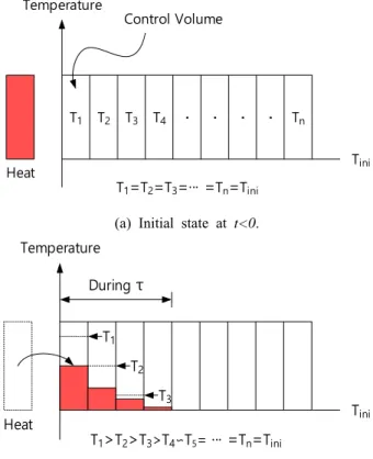
For finding the analytical solution of Equation (2), the heat transfer mechanism as shown in Figure 1 was devised. The in- itial state is shown in Figure 1 (a); the whole system is main- tained at any initial temperature (t<0). As shown in Figure 1 (b), the left surface temperature is suddenly in- creased to Thot at t=0, then the heat flow will be caused by the temper- ature gradient between both surfaces of the first shell.
The heat energy flowed into the 1st shell will increase its own temperature and creates the temperature difference be- tween itself and the 2nd shell. The created temperature gradient between the 1st and the 2nd shells causes another heat flow.
Certainly, these two procedures, which are the temperature rise of itself and the heat transfer to the neighboring shell under an initial temperature, will be occurred at the same time.
The 1st shell consumes a part of the inflow heat for its own temperature raise and transfers the rest of it to the 2nd shell.
Due to the heat transferred from the 1st shell, the 2nd shell will also raise its own temperature and transfer a part of it to the 3rd shell and so on.
Temperature
Control Volume
Tini
Heat
T1 T2 T3 T4 Tn
T1=T2=T3=··· =Tn=Tini
· · · ·
(a) Initial state at t<0.
Temperature
Tini Heat
T1 T2
T3
T1>T2>T3>T4∽T5= ··· =Tn=Tini During τ
(b) Transient state from t=0 to t=τ.
Figure 1: Heat transfer mechanism due to a thermal disturbance. (a) An initial state, which is maintained at a constant temperature, Tini, while (b) presents the transient state during t=0 to t=t. At t=0, the temperature of the left surface of the system suddenly increased. The subsequent heat transfer rates will be reduced because the former con- trol volume will consume a part of the heat transferred to increase its temperature, while the rest of it is transferred to neighboring shells.
Tini
Temperature
Thot
Length System Length
Sudden Change at t=0
Initial Temperature t<0 t Increase
Figure 2: Predicted variation of a temperature profile with time. A sudden temperature increase is applied to the left surface of a system at t=0. Referring to Figure 1 (b), the temperature gradient exponentially approaches a non-equili- brium steady state when the right surface is maintained at the initial temperature, Tini.
However, comparing the inflow heat to the 1st shell with the inflow heat to the 2nd shell, the latter will be smaller than the former since the 1st shell consumed a part of inflow heat for the temperature rise of itself as shown in Figure 1 (b). This behavior will be continued, however some shells at some dis- tance away from the 1st shell don’t perceive these thermal transient at the upstream region at all because the heat en- ergies transferred through the shells will be gradually reduced, which means that the temperature increases in the shells will be also pro- gressively smaller.
From the physical intuition, the temperature profiles will be varied exponentially as shown in Figure 2. Since the heat transfer rates among the shells are consecutively reduced, each shell faces with the situation to increase its own temperature and transfer the remain heat energy to the next shell.
Therefore, it is natural to pick up the exponential function for an analytical solution for Equation (2) although the authors had suffered from many trials and errors to find a sui- table type of function. Finding an analytical solution was started with polynomial function consisting of time and displacement, trig- onometric functions, and then power series and so on.
2.2 Mathematical solution of the C-V equation
Since the temperature of a system is varied along the spatial and the time coordinates, the solution of Equation (2) will in- clude the two independent variables of x and t, that is, T=T(x,t). In order to incorporate the variables x and t to the exponential function as a possible solution, the form of Equation (4) is selected.
(4)
In Equation (4), A, a and b, are the arbitrary constants at the present status. From the inspection of the proposed sol- ution, a and b have units of m-1 and t-1, respectively, because the exponential function will only take numeric values. This means that the constant A has to be the temperature, although the exact values of these constants are not known at this stage.
After partial differentiation of Equation (4) with respect to x and t, and substitution of the partial derivatives into Equation (2), the following condition is obtained.
(5)
In Equation (5), CT2 is /and its square root is the ther- mal wave propagation speed mentioned in Section 2.
Cancelling the common factor that exists in both sides of
Equation (5), Equation (6) is obtained.
(6)
From the inspection of each term of Equation (6), it is con- firmed that their units are identical to s-2, and maintain the di- mensional homogeneity. In order for Equation (4) to qualify as a potential solution for the partial differential equation of Equation (2), the condition of Equation (6) must be satisfied.
For finding the values of A, a and b, of Equation (4), the two boundary conditions are applied to it: T(x,t)=Th at t=0 and x=0; T(x,t)=Ti at t=0 and x=l, where l is the length of a system, as shown in Figure 2.
Use of the two boundary conditions, allows the determi- nation of the two unknown constants.
(7)
(8) From Equation (7) and Equation (8), it is found that A is simply the temperature change imposed on a boundary, and a has the units of m-1. Therefore, the requirements for the appro- priate units for A and a are satisfied. Since the value of b is calculated from the quadratic formula of Equation (6), the two unknown values will be obtained.
(9)
(10)
From the inspection of Equation (9) and Equation (10), the unit of b is still s-1, which is consistent with the requirement for selecting Equation(4) as the potential solution for the C–V equation [Equation (2)].
Although b can take values as indicated by the two cases of Equation (9) and Equation (10), there would be no problem to find a general solution if the superposition principle is ap- plied to the particular solutions that have been obtained [18].
In order to apply the superposition principle, the general sol- ution of Equation (2) will be given as follows.
(11)
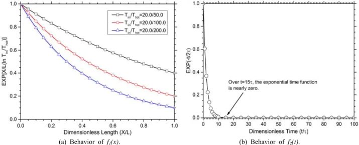
(a) Behavior of f1(x). (b) Behavior of f2(t).
Figure 3: The behaviors of the exponential functions of Equation (13) and Equation (14) that are incorporated in the general solution of Equation (12) used for the solution of the C–V equation. From (b), when the time is 15 times (or more) the ther- mal relaxation time, t, the value of f2(x) is nearly zero. It should be noted that the value of f2(x) is not exactly zero mathe- matically, but practically it can be treated to be equal to zero.
3. Analytical solution
Substitution of the determined constants of Equation (7), Equation (8), Equation (9), and Equation (10), into Equation (9), the analytical solution of Equation (11) takes the following final form:
×
(12)
In Equation (12), there are four exponential terms, which are all functions of x and t. Prior to the calculation, the following functions were investigated in order to assess their characteristics.
(13)
(14)
(15)
(16)
Figure 3 (a) shows that the transient temperature change that occurs at the boundary progressively decreases as the dis-
tance from the boundary increases. This behavior is remark- able when the temperature difference, T=Th-Ti, becomes larger. However, since the form of the exponential, spatially varying function, is continuous, it will be never become zero.
Figure 3 (b) shows the behavior of the temporally varying exponential function. One of its features is that even at a time equal to (or larger than) approximately 15 times the di- mensionless time t/ the function does not reach zero, but practically it can be treated as zero. This feature of the ex- ponential function implies that the heat penetration depth could be approximately equal to the thermal wave speed times 15.
Equation (15) and Equation (16) can be identified only if the values of , , l, Ti and Th have to be given. Generally, the thermal diffusivities of materials have values within the range of 10-3 to 10-6 m2/s. However, many arguments have been posed for the values of the thermal relaxation time. It is re- ported that it takes values in the range from 10-8 to 10-12 s, except in the case of biological tissues [19]-[21].
Figure 4 shows the variations of Equation (15) and Equation (16) with the dimensionless time, t/, in which the term multi- plied by t∙a in the square root was ignored because it is the constant determined by the material properties and the con- ditions imposed to a system. From this figure, it can be pre- dicted that the general solution of Equation (12) will show an unrealistic physical situation because Equation (15) has the characteristic of a sharply increased function with a time. This unacceptable behavior is resulted from the shape of Equation (15), which is the exponential function to be increased con- tinuously with a time.
Figure 4: The The characteristics of Equation(15) and Equation(16) included in the general solution of Equation(12). The term multiplied by ∙in the square root was ignored because it is constant.
If Equation (12) is accepted as the general solution with- out any manipulation, the temperature of the surface that is in contact with a heating or a cooling source is equal to two times the temperature of any transient source, an out- come which results from the fact that the values of Equation (15) and Equation (16) are the unit values at t=0, as seen in Figure 4.
Inspection of the behaviors of Equation (15) and Equation (16) in Figure 4 indicates that the former increases with time, while the latter decreases to zero, and the effect disappears over 5. Therefore, it would be reasonable that Equation (16) should be excluded from the general solution of Equation (12) because it approaches zero with increasing time. In order to exclude the term that is not inconsistent with the actual phys- ical phenomenon, this operation is usually applied to the pro- cedure to find the solutions of specific differential equations [18]. Thus, the final form of the general solution for the non-Fourier’s heat conduction of Equation (2) is determined as follows:
×
(17)
To investigate the features of the suggested general sol- ution for the C–V equation, the values of and should be known a priori. From the references [19]-[21], the val- ues of the thermal relaxation time in metals range from 10-8 to 10-12 s. These are extremely small values, taking into account a typical heat transfer process. If this range of
is inserted into Equation (17), the calculated values of the exponential functions may yield tremendously large positive or negative values, which will not allow easy de- lineation of the features of the obtained general solution.
To avoid this, the experimental data generated by K. Mitra et al. [22] are referred in this study, and they are repro- duced in Table 1.
Table 1: Experimentally measured thermal properties of processed meat [22]
Material ρ
(kg/m3)
cp
(J/kg·K)
k (W/m·K)
α (m2/s) Processed
Meat 1230 4660 0.8 1.4*
* 10-7 shall be multiplied.
Note 1: Test range is about 6 oC to 29oC.
Note 2: Experimental uncertainties in the original study are not included in this table.
Note 3: Measured thermal relaxation time is distributed in 15~16 seconds.
The used values for the calculation are =15 s and
=1.4x10⁻⁷ m2/s. The length of a specimen and the initial temperature are assumed to be 20 mm and 20 °C, respectively.
Assume that beef with a thickness of 20 mm is used to cook a steak using a hot grill that is assumed to maintain the tem- perature of 160 °C at all times. In addition, natural convection that occurs owing to the temperature difference between the meat and the ambient temperature over its upper and side sur- faces is ignored.
Figure 5 (a) shows the temperature variations in the meat that is placed on a hot grill at specific positions, which are 1 mm, 2 mm, and 3 mm from the hot surface, during the period of 5. Numerically, the temperature rise in the cooked meat is increased at small distances away from the hot surface.
However, the changes are not. This variation results from the large value of the thermal relaxation time, and the selected po- sitions that are too close to each other.
Figure 5 (b) shows the temperature variations with time, and the forced constraint is applied to the heated boundary.
Its temperature was set at 160 °C, while the natural con- vection from the opposite surface was ignored. This figure clearly shows that the temperatures of the meat are in- creased as time progresses. Even though the extent of the temperature rise is not remarkable, the change in temper- ature probably resulted from the large value of the thermal relaxation time.
(a) Temperature variations in cooked meat as a function of position
(b) Temperature variations of cooked meat as a function of time Figure 5: Calculated temperatures in meat. The data described in Table 1 were used for calculation. In the case of (a), three spatial locations are selected from the heated boundary surface, namely 1 mm, 2 mm, and 3 mm. In the case of (b), the temporally varying temperature variations in meat are shown. Clearly, the temperatures in meat increase as the time progresses.
4. Conclusion
The purpose of the study was the identification of a simple type of a general solution for the hyperbolic partial differential equation of the non-Fourier’s heat conduction, known as the C –V equation. Up to now, many studies have suggested the use of analytical solutions for the C–V equation. Even though con- sideration of this equation may accurately predict the transient state of a system, the elicited outcomes have very complicated shapes. This fact constitutes a barrier to users without ex- tensive mathematical knowledge or skills.
The introduced concept in this study for bypassing the math- ematical complication is to assume a simple solution, and con- firm whether the assumed solution satisfies the originally given
differential equation. Through numerous empirical tests of vari- ous functions, the simple exponential function of Equation (4) was confirmed to satisfy mathematically the non-Fourier differ- ential equation of Equation (2). However, the behavior of the general solution elicited unrealistic temperature profiles in the virtual experiment using published experimental data.
Although it is verified in this study that the general solution of Equation (12) satisfies the hyperbolic partial differential equation used for the non-Fourier’s heat conduction, but is somewhat defective from a practical viewpoint. In view of these facts, the term of Equation (16) was excluded from the general solution since it revealed the temperature profile that is inconsistent with common sense, and therefore the final form of the general solution was determined in accordance to Equation (17).
However, the authors have no assurance on whether the ex- cluded term of Equation (16) is actually unrealistic or whether it contains any other meaning not perceived by the authors.
Certainly, it maintains the initial temperature at the beginning of a transient state, and its effect disappears with time, which resembles the effect of thermal inertia resisting an imposed thermal disturbance.
From the calculated results, all temperatures at the various positions in cooked meat elicited higher temperatures than the initial temperature that increased with time. However, the gen- eral solution continuously increased with time.
As described in the introduction, this study is the first trial to identify a simple type of an analytical solution of the non-Fourier’s heat conduction phenomena. It was performed to confirm the possibility on whether or not a simple exponential function can be used as the solution for the C–V equation.
According to this viewpoint, the results of this study provide initial evidence to the adopted approach for a simple type of a general solution for the C–V equation.
References
[1] O. Kwon, L. Shi, and A. Majumdar, “Scanning ther- mal wave microscopy (STWM),” ASME Journal of Heat Transfer, vol. 125, no. 1, pp. 156-163, 2003.
[2] C. A. Nanni and T. S. Alster, “A practical review of laser-assisted hair removal using the Q-switched Nd:
1/AG, long-pulsed ruby, and long-pulsed alexanvlrite Lasers,” Dermatologic Surgery, vol. 24, no. 12, pp.
1399-1405, 1988.
[3] D. D. Joseph and Luigo Preziosi, “Heat Waves,” Review of Modern Physics, vol. 61, no. 1, pp. 41-73, 1989.
[4] K. K. Tamma and X. Zhou, “Macroscale and micro-
scale thermal transport and thermo- mechanical inter- actions: Some noteworthy perspectives,” Journal of Thermal Stresses, vol. 21, no. 3-4, pp. 405-449, 1988.
[5] C. J. Cho and W. N. Juhng, “Non-fourier heat con- duction in a slab subjected to periodic surface heat- ing,” Journal of Korean Phisical Society, vol. 36, no.
4, pp. 209-214, 2000.
[6] R. Eisberg and R. Resnick, Quantum Physics of Atoms, Molecules, Solids, Nuclei and Particles, New York, USA: John Wiley & Sons, 1985.
[7] A. Salazar, “Energy propagation of thermal waves,”
European Journal of Physics, vol. 27, no. 7, pp.
1349-1355, 2006.
[8] M. N. Ozisik and D. Y. Tzou, “On the Wave Theory in Heat Conduction,” ASME Journal of Heat Transfer, vol. 116, no. 3, pp. 526-535, 1994.
[9] M. N. Ozisik and Brian Vick, “Propagation and re- flection of thermal waves in a finite medium,”
International Journal of Heat and Mass Transfer, vol.
27, no. 10, pp. 1845-1854, 1984.
[10] M. Chester, “Second sound in solids,” Physical Review, vol. 131, no. 5, pp. 2013-2015, 1963.
[11] J. Gembarovic and V. Majernik, “Non-fourier prop- agation of heat pulses in finite medium,”
International Journal of Heat and Mass Transfer, vol.
31, no. 5, pp. 1073-1080, 1988.
[12] X. Ai and B. Q. Li, “Numerical simulation of ther- mal wave propagation during laser processing of thin films,” Journal of Electronic Materials, vol. 34, no. 5, pp. 583-591, 2003.
[13] J. Shiomi and S. Maruyama, “Non-fourier heat con- duction in a single walled carbon nanotube: Classical molecular dynamics simulations,” Physical Review B, vol. 73, no. 20, pp. 205420-1-205420-7, 2006.
[14] C. W. Chang, D. Okawa, H. Garcia, A. Majumdar, and A. Zettl, “Breakdown of fourier’s law in nano- tube thermal conductors,” Physical Review Letters, vol. 101, no. 7, pp. 075903-1-075903-4, 2008.
[15] M. Jaunich, S. Raje, K. H. Kim, K. Mitra, and Z.
Guo, “Bioheat transfer analysis during short pulse la- ser irradiation of tissues,” International Journal of Heat and Mass Transfer, vol. 51, no. 23-24, pp.
5511-5521, 2008.
[16] C. F. Jin, K. K. Kim, H. S. Chung, H. M. Jeong, D.
Y. Choi, and S. H. Choi, “A study of the heat con- duction phenomena with a phase lag of heat flux,”
Journal of the Korean Society of Marine Engineering, vol. 32, no. 5, pp. 684-690, 2008 (in Korean).
[17] D. Y. Tzou, Macro- and Micro-scale Heat Transfer, Washington DC, USA: Taylor & Francis, 1996.
[18] E. Kreyszig, Advanced Engineering Mathematics, New York, USA: John Wiley & Sons, 1988.
[19] P. K. L. Chan, K. P. Pipe, Z. Mi, J. Yang, P.
Bhattacharya, and D. Lüerßen, “Thermal relaxation time and heat distribution in pulsed InGaAs quantum dot lasers,” Applied Physics Letters, vol. 89, no. 1, pp. 011110-1-011110-3, 2006.
[20] Z. Y. Ong and E. Pop, Molecular Dynamics Simulation of Thermal Boundary Conductance be- tween Carbon Nanotubes and SiO2, Phys. Rev. B, vol. 81, no. 15, pp. 155408-1-155408-7, 2010.
[21] J. Y. Lin, “The non-fourier effect on the fin performance under periodic thermal conditions,” Applied Mathmatical modelling, vol. 22, no. 8, pp. 629-640, 1988.
[22] K. Mitra, S. Kumar, A. vedavarz, and M. K.
Moallemi, “Experimental evidence of hyperbolic heat conduction in processed meat,” ASME Journal of Heat Transfer, vol. 117, no. 3, pp. 568-573, 1995.
![Table 1: Experimentally measured thermal properties of processed meat [22] Material ρ (kg/m 3 ) c p (J/kg·K) k (W/m·K) α(m2 /s) Processed Meat 1230 4660 0.8 1.4* * 10 -7 shall be multiplied.](https://thumb-ap.123doks.com/thumbv2/123dokinfo/4824987.281236/6.892.93.426.128.372/experimentally-measured-thermal-properties-processed-material-processed-multiplied.webp)
