A Study on Flow Characteristics of Polluted Air in Rectangular Tunnel Models Using a PIV System
Young-Ha Koh†․Sang-Kyoo Park1․Hei-Cheon Yang1․Yong-Ho Lee1 (Received Mar. 27, 2010; Revised Aug. 16, 2010; Accepted Sept. 27, 2010)
Abstract: The objective of this study is to investigate flow behaviors of polluted air in order to prevent the impact of disaster in a tunnel. This paper presents the experimental results qualitatively in terms of flow characteristics in two kinds of rectangular tunnel models in which each distance from the centerline above the inlet vent to the exhaust vent is 0 and 60 mm, respectively. The olive oil is used as the tracer particles. The flow is tested at the flow rate of
× m
s and the inlet vent velocity of 1.1 ms with the kinematic viscosity of air. The aspect ratio of the model test section is 10. The average velocity vectors, streamlines, and vorticity distributions are measured and analyzed by the Flow Manager in a particle image velocimetry(PIV) system. The PIV technology gives three different velocity distributions according to observational points of view for understanding the polluted air flow characteristics. The maximum value of mean velocity generally occurs in the inlet and outlet vent regions in the tunnel models.
Key words: PIV, average velocity vector, streamlines, vorticity, Flow Manager
†Corresponding Author(Dept. of High-tech. CAD/CAM, Chosun College University of Science &
Technology)
1 College of Engineering Science, Chonnam National University (Yeosu Campus)
1. Introduction
In tunnels, pollutants are released by automobiles and other powered vehicles, even though there are many emission standards that set specific limits to the amount of pollutants. The standards regulate the emissions of nitrogen oxides, sulfur oxides, particulate matter or soot, carbon monoxide, or volatile hydrocarbons.
In case of fire in underground tunnels, ventilation and smoke-extraction systems are the dominant factors for the safety requirements to evacuate a large number of passengers or workers.
The earliest quantitative velocity
measurements in fluid flows were obtained
using Pitot-static tubes[1]. Following this
early stage of velocity measurement tools,
the constant temperature hot-wire
anemometry had permitted by the
introduction of high technology in optics
and electronics[2]. The invention of the
laser in the 1960s led to the development
of laser Doppler velocimetry. Liou et
al[3]. observed mean velocities,
turbulence intensities and Reynolds
stresses by LDV in a rectangular tunnel
at a Reynolds number of 33,000. With the
utilization of laser-Doppler anemometers,
numerous studies have been presented by
Halim (1988) [4] ana Meyer Larsen (1994) [5] in order to provide detailed mapping of velocity fields. Hirleman and Naqwi et al [6,7]. contributed much to the development of phase-Doppler anemometry and the application of PDA systems to study laminar and turbulent two-phase flows. Hirota et al [8]. performed the secondary flow patterns caused by perpendicularly arranged square ribs in a square duct. However, most available data were limited to perpendicular ribs in square ducts or high aspect ratio rectangular ducts at high Reynolds numbers. In addition, it has the limitation that it can not capture the simultaneous spatial structure of a flow field.
Particle image velocimetry (PIV) employs an optical setup to observe the characteristics of the flow structure in a rectangular tunnel in this paper. PIV is a whole flow field technique providing components of the velocity fields by a scattering particle. To have instantaneous velocity vector measurements in a cross-section of a flow, enough light is scattered by the corresponding particle. It is possible to obtain instantaneous velocity maps in a flow plane of interest.
By post-processing, the mean velocity maps and instantaneous or average vorticity maps can be obtained [9,10]. PIV has matured from its developmental stage to a reliable whole field flow measurement technique and continuously enlarged the boundaries of scientific applications. PIV systems for the investigation of air flows in wind tunnels must be capable of recording low speed flows [11] (e.g. flow velocities of less than 1 m/s in turbulent boundary layers) as well as high speed
flows with flow velocities exceeding 500 m/s. Flow fields above solid, moving or deforming models are also frequently associated with flow reversals. The application of the PIV technique in large, industrial wind tunnels poses a number of special problems: large observation areas, large observation distances between camera and light sheet, time constraints in the setup of the PIV system, and high operational costs of the wind tunnel [12].
This paper presents the experimental results of air flow such as velocity field, streamline field and vorticity in the rectangular tunnel which has the different locations of the exhaust outlets. The main objective of this paper is to investigate the flow characteristics qualitatively in a rectangular tunnel model by using PIV.
The thermal characteristics are not taken into consideration in this study. However, it will be expected to minimize the damage caused by toxic substance in road and subway tunnels and help other pollutants including smoke to be properly vented to the outdoors.
1.1 Similarity
In road or underground tunnels, it is
mostly not reasonable to model the whole
tunnel because of the extremely high
aspect ratio of typical tunnels. For the
Monte Blanc tunnel with a hydraulic
diameter of 7 m and a length of 11.6 km,
it is 1657 [15]. It might not be
reasonable to consider this ratio as a vital
factor. However, in this study the aspect
ratio of the test section is 10, and
therefore the real length of a tunnel is
800 m for a hydraulic diameter of 8 m. It
could be a similar length in many Korean
road tunnels.
The experiment in this study was conducted at the same velocity and at a Reynolds number of 5830. Other papers [14,15] presented the results and discussions according to the variation of Reynolds numbers. In addition, it is necessary to make three-dimensional, instantaneous and simultaneous flow measurements of the four main fluid variables: temperature, density, pressure, and velocity. However, there is no temperature difference between atmospheric air and olive oil particles defined as polluted air. Consequently, the velocity fields are mainly focused on in this paper according to different vent positions. If a smoke source along with temperature and density is considered, the Froude Number should be dealt with.
2. Experiment
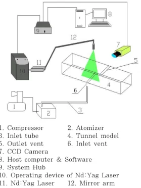
The experiment equipments are made up of four basic components: (1) An optically transparent test-section containing the flow seeded with tracer particles; (2) A light source (laser) to illuminate the region of interest (plane or volume); (3) Recording hardware consisting of either a CCD camera, or film, or holographic plates; (4) A computer with suitable software to process the recorded images and extract the velocity information from the tracer particle positions. The experiment equipments are shown in Figure 1.
The transparent acrylic rectangular tunnel of the test section is presented in Figure 2. The length, height and width of the tunnel model is 800 mm, 80 mm, and
80 mm, respectively. As shown in Figure 2, the inlet vent is positioned in the middle of the tunnel bottom, while the outlet vents are located at two different positions at the top of the tunnel.
1. Compressor 2. Atomizer 3. Inlet tube 4. Tunnel model 5. Outlet vent 6. Inlet vent 7. CCD Camera
8. Host computer & Software 9. System Hub
10. Operating device of Nd:Yag Laser 11. Nd:Yag Laser 12. Mirror arm
Figure 1: A schematic of experimental equipments.
Figure 2: The test section of the experiment.
(L= 0 and 60 mm)
The distance between the inlet and
outlet vent is specified as L = 0 and 60
mm. The width and length of the inlet
and outlet vents is 30 mm and 80 mm, respectively. The olive oil particles supplied by an air compressor are atomized to the test section. Those particles are flowed into the rectangular tunnel through the plastic-pipe and then exit through the upper outlet vent. In order to get the appropriate flow speed, a plastic-trunk is used for lower speeds and a small axial flow fan is installed to provide uniform flow. Each image is captured by the CCD camera which is positioned at right angle to the light-sheet in the Dantec PIV 2000 system. The image corresponds to two pictures. The picture A is taken at time T and the picture B is taken at time T+ t, where t depends on the time between pulses. Then the pictures are transferred to the PIV processor software Flow Manager.
In this software, for reasons of experimental reproducibility, the raw vector maps are archived and a new validated vector maps are offered. Further analysis can produce streamlines, vorticity distribution, velocity distribution, and instantaneous kinetic energy.
3. Results and discussions
In this experiment, the experimental flow is an atomizing smoke at the same speed and the same thickness, using the jet fan to control and change the speed of the smoke flow in the tunnel. The olive oil has been used as the tracer particles and the kinematic viscosity of the air flow is ×
m
s .
3.1 The average velocity vector fields and streamlines The polluted air flow characteristics
have been tested at the flow rate of 5.1 m
h and the velocity of 1.1 m/s through the inlet like the smoke source. In order to show the flow velocity fields at the inlet and outlet vents, the cross-sectional image of 145 mm × 80 mm area as a test section has been examined by using PIV.
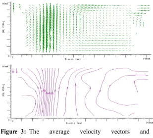
Figures. 3 and 4 demonstrate the image of distribution of average velocity produced by PIV test analysis. Figure 3 reveals the average velocity vector graph as well as the streamlines at the cross section of the tunnel. When the exhaust outlet is just at the top of the inlet position, the polluted air out of smoke sources goes upward in the upwind direction over the inlet point, and circulation flows occur near both sides of the inlet region.
Figure 3: The average velocity vectors and streamlines at L = 0 mm
As the toxic air propagation goes away from the inlet point region in the y-direction, the diffusion and emission of pollutants have not significantly changed.
These polluted air paths are assumed to
be positioned just above the inlet vent
due to the exhaust vent on the ceiling tunnel. The outlet vent, the exhaust device installed on the top of the inlet point, is conducive to people who stay in the longitudinal direction of the tunnel for an emergency escape route.
Figure 4: The average velocity vectors and streamlines at L = 60 mm
As shown in Figure 4, the fluid circulation is being produced from the flow toward the right side of inlet position due to the impact of the tunnel wall. The outlet vent is located at 60 mm away on the right side compared with the previous vent in Figure 3. At the same time, one large circulation flow is found at the right bottom region under the exhaust vent in the tunnel. This implies that some part of flow along the ceiling layer is exhausted into the outlet vent and the rest of the flow goes inside the tunnel due to the tunnel ceiling. It is also observed that the maximum value of mean velocity occurs in the inlet and outlet vent regions. It is helpful to decide valid methods of toxic gas emissions and to save endangered people by estimating flow characteristics toward the windward or leeward direction
in the tunnel. The flow velocity at the upper part of the tunnel is significantly larger than that of the lower part.
Increasing the longitudinal flow velocity makes the polluted air spread to the leeward direction.
3.2 Mean Vorticity Distribution
Figure 5 shows mean vorticity distribution in the tunnel of the L = 0 mm case. The vortices are longitudinally found, since the inlet and the outlet vents are located at the same in the x direction, as shown in Figure 2. The high vorticity has been formed along the streamlines from the inlet source. On the other hand, the low vorticity has built up just beside the high one at the same time. In Figure 6, a little high vorticity has been formed near the inlet area. It is assumed that the change of the streamlines due to moving to the exhaust vent at L=60 mm should make the vorticity low in the limited space inside the tunnel. The vortices are generally active near the lower part of the tunnel from the inlet region.
Figure 5: Mean vorticity distribution at L = 0 mm
Figure 6: Mean vorticity distribution at L = 60 mm
3.3 Three Different Velocity Distributions According to Observational Points of View
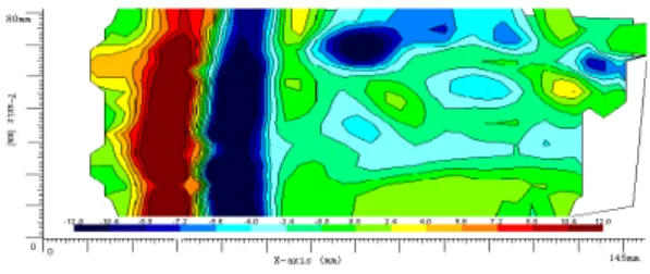
Contour pl ot i s the basi c type of visualization for analyzing the scalar and vector fields according to field value in each contour. Figs. 7 and 8 present contour plots of velocity magnitude derived from the velocity fields according to the different positions of the outlet vent by using PIV measurement. Figure 7 shows the velocity contours of the flow fields of polluted air qualitatively from three different viewpoints at L = 0 mm.
The regions of high mean velocity are driven into the one domain, which starts
(a) Contours of mean velocity
(b) Contours of x-component velocity
(c) Contours of y-component velocity Figure 7: Velocity distributions obtained from three different viewpoints on the smoke velocity field at L
= 0 mm
(a) Contours of mean velocity
(b) Contours of x-component velocity
(c) Contours of y-component velocity Figure 8: Velocity distributions obtained from three different viewpoints on the smoke velocity field at L=60 mm
from the inlet vent to the outlet, as
shown in Figure 7(a). Even though the
magnitude of - component velocity is
very lower than that of mean velocity, the
contour plots of mean velocity and
-component velocity are similar in flow
patterns. On the other hand, the pattern
in - component velocity contour is
different from those of two previous
velocity contours due to the flow velocity
difference caused by the flow direction in
the same flow field. The magnitude of
-component velocity is lowest. It means
that the flow in the - direction has not
any specific effect on the tunnel flow.
Figure 8 shows the three velocity contour plots obtained from the different viewpoints regarding the flow fields in the L = 60 mm case. As the outlet vent is placed at 60mm away from the centerline, the high velocity region is reduced compared to the case of L=0 mm in the meantime and the realm of -component velocity moves off from the centerline to the outlet vent. It is conducive to people who stay in the leeward direction to escape. In this case the effect of smoke emission is more evident. Both the high velocity regions in the -component, as shown in Figs. 7(b) and 8(b), are positioned at the ceiling in the tunnel.
4. Conclusions
This study has qualitatively produced velocity vectors and streamlines, mean vortices, and three different velocity distributions in two kinds of rectangular tunnel models. The two test models of L
= 0 and 60 mm are investigated and analyzed regarding flow characteristics under the same experimental conditions in a comparative way.
(1) The maximum value of mean velocity generally occurs in the inlet and outlet vent region. The flow velocity at the upper part of the tunnel is significantly larger than that of the lower part.
Increasing the longitudinal flow velocity makes the air spread to the leeward direction. It is conducive to keep away from the realm of toxic air pollutants and to let people get out of danger toward the windward direction.
(2) The contour plots of mean velocity and component velocity are similar in
flow patterns even though the magnitude of component velocity is very lower than that of mean velocity. On the other hand, the pattern in component velocity contour is different from those of two previous velocity contours due to the flow velocity difference caused by the flow direction in the same flow field.
(3) The vortices are generally active near the lower part of the tunnel from the inlet region. Finally, the maximum value of the energy in the L = 60 mm case is located near the exhaust vent and is generally lower than that in the L = 0 mm case. These results are presumed to occur because both end-sides of the tunnel are naturally ventilated in the testing room. Further studies are needed to investigate and discuss pressure distributions and other thermal quantities using PIV and CFD.
References
[1] Ajay K. Prasad, Particle image velocimetry, Department of Mechanical Engineering, University of Delaware, Newark, DE, 103-116, 2000.
[2] Bruun, H.H., Hot - Wire Anemometry:
Principles and Signal Analysis, Oxford University Press Inc. New York, 1995.
[3] T.M. Liou, Y.Y. Wu, Y. Chang, LDV measurements of periodic fully developed main and secondary flows in a channel with rib-disturbed walls, ASME J. Fluids Eng. 115(1) 109-114, 1993.
[4] Halim, Detailed velocity measurement
of flow through staggered and in-line
tube banks in cross-flow using laser
Doppler anemometry. Ph.D. thesis,
University of Manchester. 23-56, 1988.
[5] Meyer, K.E. and Larsen, P.S., "LDA study of turbulent flow in a staggered tube bundle", 7th Int. Symp. on Applications of Laser Techniques to Fluid Mechanics, Lisbon, paper 39.4, 1994.
[6] Hirleman, E.D., "History of development of the phase-Doppler particle-sizing velocimeter", Part. Charact. 13, pp.
59-67, 1996.
[7] Naqwi, A., Durst, F., Liu, X., "Two optical methods for simultaneous measurement of particle size, velocity and refractive index", Applied Optics, vol.30, no.33, pp.4949-4959, 1991.
[8] M. Hirota, H. Fujita, H. Yokosawa,
"Experimental study on convective heat transfer for turbulent flow in a square duct with a ribbed rough wall (characteristics of mean temperature field)", ASME J. Heat Transfer 116 (2) 332-340, 1994.
[9] M. Raffel, C. Willert, J. Kompenhans, Particle Image Velocimetry, A Practical Guide, Springer, 88-123, 1998.
[10] Dantec Dynamics, Flow Manger software and introduction to PIV: 2D PIV Installation and User's Guide, 33-118, 2000.
[11] R. J. Adrian, Twenty years of particle image velocimetry, Experiments in Fluids 39: 159–169, 2005.
[12] Grant I. Particle image velocimetry, A review, Proceedings Institute of Mechanical Engineers, 211, pp. 55-76, 1997.
[13] Marco Bettelini, HBI Haerter AG, Zurich, "CFD for tunnel safety", FLUENT Users' Meeting, Bingen,
2001.
[14] Sang-Kyoo Park, Hei-Cheon Yang, Yong-Ho Lee, Gong Chen, "PIV measurement of the flow field in rectangular tunnel", J. of the Korean Society of Marine Engineering, vol.
32, no.6, pp. 886-892, 2008.
[15] Yong-Ho Lee, Sang-Kyoo Park, "Flow field analysis of smoke in a rectangular tunnel", J. of the Korean Society of Marine Engineering, vol.
33, no.5, pp. 679-685, 2009.
Author Profile
Young-Ha Koh
Professor, Dept. of High-tech.
CAD/CAM, Chosun College University of Science & Technology : Ph.D. in Mechanical Eng. Chosun Univ. in 1992, M.S. in Mechanical Eng. Chosun Univ.
in 1987.
Sang-Kyo Park
Professor, College of Engineering Science, Chonnam National Univ.
(Yeosu Campus): Ph.D. in Mechanical Eng. Inha Univ. in 1989, M.S. in Mechanical Eng. Inha Univ. in 1983.
Hei-Cheon Yang
Professor, College of Engineering Science, Chonnam National Univ.
(Yeosu Campus): Ph.D. in Mechanical Eng. Chung-Ang Univ. in 1994, Born in February 1961.
Yong-Ho Lee
Instructor, College of Engineering Science, Chonnam National Univ.
(Yeosu Campus): Ph.D. in Mechanical Eng. Chonnam National Univ. in 1999, M.S. in Mechanical Eng. Inha Univ. in 1985.