- 1759 -
신경망과 외란 추정 기법을 이용한 비선형 시스템의 적응 슬라이딩 모드 제어
이재영*, 박진배*, 최윤호**
연세대*, 경기대**
Adaptive Sliding Mode Control of Nonlinear Systems Using Neural Network and Disturbance Estimation Technique
Jae Young Lee*, Jin Bae Park*, Yoon Ho Choi**
Yonsei University*, Kyonggi University**
Abstract - This paper proposes a neural network(NN)-based adaptive sliding mode controller for discrete-time nonlinear systems.
By using disturbance estimation technique, a sliding mode controller is designed, which forces the sliding variable to be zero. Then, NN compensator with hidden-layer-to-output-layer weight update rule is combined with sliding mode controller in order to reduce the error of the estimates of both disturbances and nonlinear functions. The whole closed loop system rejects disturbances excellently and is proved to be ultimately uniformly bounded(UUB) provided that certain conditions for design parameters are satisfied.
1. Introduction
Adaptive control has been studied by many researchers, due to its capability of reducing parametric uncertainties and thus to improve the performance while the stability of the closed loop system is guaranteed [1]. In the past several years, there are many studies to use neural network(NN) as a part of online discrete-time adaptive controllers [2][3][4]. The purpose of the use of NN is to approximate uncertain part of systems or controller continuously, thus, to improve the performance of the close loop system.
On the other hand, sliding mode control(SMC) in discrete-time system has more attention recently due to the numerous use of digital computer and its robustness property[5][6]. Among various discrete-time sliding mode controller, disturbance-estimation-based sliding mode controller[6] improves its performance by providing estimates of disturbances with small error. However, the small error is still exist and can deteriorate the system performance. Furthermore, in [6], the controller is designed only for the linear time-invariant (LTI) systems, not for nonlinear systems.
In this paper, we extend the above sliding mode controller to the control of nonlinear systems where the disturbances and nonlinear functions are completely unknown. In addition, NN is used to compensate the remaining estimation error, thus to improve control performance. The proposed controller estimates both of the disturbances and nonlinear functions by using disturbance estimation technique [6]. Then, NN with promising update rule is used as a compensator, which reduces the effect of estimation errors and uncertainties, and gives robustness to disturbances. Furthermore, the proposed controller is proved to be UUB with learning rate and control gain constraint, and, thus, guarantees boundedness of all the signals. Simulation result shows good tracking performance as well as its stability and robustness in the uncertain environment.
2. Main Discourse
2.1 Problem Formulation
Consider the following class of discrete-time nonlinear systems in Brunovsky canonical form:
(1)
where the vector ⋯ ∈ with each column vector ∈ is the state at time
instant k, ∈ is the system input, and ∈ is the external matched disturbance, respectively. Here we assumed that 1) the states are measureable for all time instant ≥ , and 2) the function f(x(k)) and the disturbance d(k) are unknown.
Define tracking error as where
and is the desired trajectory of .
2.2 NN-Based Adaptive Sliding Mode Controller Design
Define the sliding surface as
(2)
where K1, ... , Kn-1 is gain matrix, designed such that the transfer matrix from s(k) to en(k) is Hurwitz; is defined as
. The controller which yields stable LTI system s(k+1)=Hs(k) is designed as follows:
(3)
⇒ . (4) where ∈ × is the Hurwitz gain matrix. Since we have assumed that f(x(k)) and d(k) are unknown, we cannot use the above controller (4). Instead, the one-step-before value f(x(k-1)) + d(k-1) can be obtained by (2) as (see [6])
. (5) Therefore, instead of using the exact values of f(x(k)) and d(k), the one-step-before value f(x(k-1)) + d(k-1) can be used as a estimates of f(x(k)) + d(k).
Finally, the control law u(k), combined with the above estimates and neural network compensator, is obtained as follows:
≈
∆ ∆. (7) where ∆ and ∆ are estimates of ∆:=
f(x(k))-f(x(k-1)) and ∆=d(x(k)) - d(x(k-1)), respectively.
2.3 NN Representation and NN Weight Update Rule
Here, we assume that ∆ ∆ can be represented by a multilayer feedforward NN as
∆ ∆ (9) 2008년도 대한전기학회 하계학술대회 논문집 2008. 7. 16 - 18
- 1760 -
where NN input ∈ is defined as ,
; the matrix ∈× is the optimal weight of the NN,
∈ is the optimal bias weight, ∈ is the neural network reconstruction error, and ∈ ×
is the randomly- selected input-to-hidden node weight, respectively.
Assumption 1) ∆ is bounded by a constant, i.e.,∥∆∥≤ Assumption 2) and are bounded, i.e.,
∥
∥
≤ . Assumption 3) the approximation error is bounded such that ∥∥≤ ∥∆∥≤ .
Since both ∆ and ∆ are unknown, the NN estimate of
∆ ∆, denoted by ∆ ∆, is used instead of the exact value. The estimate is defined as
∆ ∆ (10) where and are the estimates of and , respectively. The weight update rules for minimizing ∆
∆ ∆ ∆ are given as
(11)
(12)
where is the learning rate of the given weights.
2.4 Stability Analysis
The stability of the above closed loop system is stated as below:
[Theorem 1] Assume that the desired trajectory is bounded.
In addition, if Assumption 1, 2, and 3 are satisfied, and the control law and weight update rule are given by (8), (11), and (12), then, the sliding variable s(k), the weights and are uniformly ultimately bounded(UUB) provided that
∥∥
and
(13)
where is the maximum singular value of H.
proof) The proof is omitted here due to space limitations 2.5 Simulation Result
The nonlinear system to be simulated is represented as
(14)
(15) where d(k) is given by
≤ . The parameters are selected as follows:
<Table 1> Parameters in the simulation
H Nh ∙ and
0.2 0.09 0.55 10 ∙ randomly selected in [0, 1]
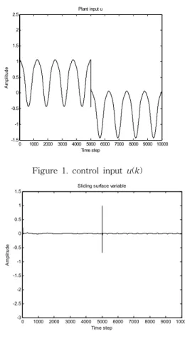
Figures 1 and 2 illustrate the simulation results of the proposed controller. As we expected, the controller excellently reduces the disturbance. The sliding variable peaks when step disturbance is applied, but reduces its amplitude very quickly, which shows good disturbance rejection.
-1.50 1000 2000 3000 4000 5000 6000 7000 8000 9000 10000 -1
-0.5 0 0.5 1 1.5 2 2.5
Time step
Amplitude
Plant input u
Figure 1. control input u(k)
0 1000 2000 3000 4000 5000 6000 7000 8000 9000 10000 -3
-2.5 -2 -1.5 -1 -0.5 0 0.5 1 1.5
Time step
Amplitude
Sliding surface variable
Figure 2. sliding variable s(k)
3. Conclusion
In this paper, a new neural network(NN)-based adaptive sliding mode controller for discrete-time nonlinear systems was proposed.
Sliding surfaces and sliding variables were defined. and then, by using the disturbance estimation technique, sliding mode controller was designed. Finally, the NN compensator with hidden-layer- to-output-layer weight update rule was designed so as to approximate the uncertain difference terms of the system. The closed loop system with proposed controller and update rule was proved to be UUB with learning rate and controller gain constraints. Simulation result showed that the proposed controller is robust and has good tracking performance.
[References]
[1] J-J E. Slotine and Weiping Li, Applied Nonlinear Control, Prentice-Hall, 1991.
[2] S. J. Yoo, J. B. Park, and Y. H. Choi, "Direct Adaptive Control using Self-Recurrent Wavelet Neural Network via Adaptive Learning Rates for Stable Path Tracking of Mobile Robots", Proceedings of the 2005 American Control Conference, pp. 288-293, 2005.
[3] S. Jagannathan and F. L. Lewis, “Discrete-Time Neural Net Controller for a Class of Nonlinear Dynamical Systems”, IEEE Trans. Automatic Control, Vol. 41, No. 1, pp. 1693-1699, 1996
[4] Pingan He and S. Jagannathan, “Reinforcement Learning Neural-Network-Based Controller for Nonlinear Discrete-Time Systems With Input Constraints”, IEEE Trans. Systems, Mans, and Cybernetics Part B, Vol. 27, No 3, pp. 425-436, 2007 [5] G. Bartolini, A. Pisano, and E. Usai, "Digital Second-order
Sliding Mode Control for Uncertain Nonlinear Systems", Automatica, Vol. 37, No 9, pp. 1371-1377, 2001.
[6] S. Janardhanan and V. Kariwala, "Multirate-Output- Feedback-Based LQ-Optimal Discrete-Time Sliding Mode Control", IEEE Trans. Automatic Control, Vol. 53, No. 1, pp. 367-373, 2008.