Dependency of hydrologic responses and recharge estimates on water-level monitoring locations within a small catchment
ABSTRACT: Estimation of groundwater recharge is essential for planning sustainable groundwater development. In this study, recharge ratios were estimated using the groundwater hydro- graphs obtained from monitoring wells located in a small catch- ment (0.256 km2). The catchment area is a triangular alluvial plain bounded by gentle hills and a large stream. For the recharge esti- mation, the modified water-table fluctuation (WTF) method was used. Although the study area is very small, the groundwater hydrographs were very different depending on the thickness of the unsaturated zone and the distance of the monitoring well from the main stream. Where the unsaturated zone is thick, the ground- water level changes smoothly in response to rainfall and resulting amplitude is small. In addition, the hydrographs closer to the stream showed quicker responses and larger fluctuations. Result- ant recharge estimates showed a very wide variation between 2.5 and 20.1%. Compared with 12.7% estimated by other study mainly based on the water budget analyses, the recharge ratios were underestimated in upgradient area (hills) while they were overestimated in downgradient area (stream). Therefore, for rep- resentative and appropriate recharge estimation based on the groundwater hydrographs, it appears that the monitoring location is most important.
Key words: recharge, groundwater level, rainfall, water-table fluc- tuation, correlation, Korea
1. INTRODUCTION
Recharge is defined in a general sense as the downward flow of water reaching the water table resulting in corre- sponding water-level rise (de Vries and Simmers, 2002).
Groundwater recharge is a critical hydrological parameter that, depending on the application, may be estimated at a variety of spatial and temporal scales (Scanlon and Cook, 2002). Many methods are available for quantifying ground- water recharge and each method has its own advantages and limitations in terms of applicability and reliability (Beek- man and Xu, 2003). Typical methods of estimating recharge ratios involve physical, tracer or numerical modeling approaches.
An appropriate method should be selected based on various factors such as hydrogeological conditions and scale of interest (Scanlon et al., 2002).
The WTF method is based on the assumption that rises in groundwater levels in unconfined aquifers are due to
recharge water arriving at the water table and is best applied to aquifer systems with shallow groundwater levels show- ing quick responses to precipitation events (Healy and Cook, 2002; Scanlon et al., 2002; Moon et al., 2004). This method involves two inherent problems: uncertainty in spe- cific yield (Sy) and effect of delayed drainage (Wilson and de Cook, 1968; Lerner, 2003). In spite of these problems, however, the simplicity of estimating recharge from hydrograph data is attractive for use wherever appropriate (Healy and Cook, 2002).
Moon et al. (2004) suggested a modified WTF method estimating groundwater recharge using the product of spe- cific yield and the ratio of water-level rise over the cumulative precipitation. They applied the modified method to water- level data obtained from the National Groundwater Monitor- ing Network of Korea and evaluated the spatial variability of recharge in river basins whose distances are at least over 20 km. Meanwhile, recharge estimates based on the WTF method can represent surface areas of 50−10,000 m2 (Scanlon et al., 2002; Beekman and Xu, 2003). Therefore, monitoring wells should be located to reflect the water levels of the aqui- fer as a whole (Healy and Cook, 2002). Water level responses to precipitation would be different at recharge and discharge areas even within a small catchment area. Consequently recharge estimates using the groundwater hydrographs at different monitoring locations are much varying.
The purposes of this study are to examine different hydrologic responses of the water levels to the same pre- cipitation events using time series analysis and to compare recharge estimates depending on the locations of the mon- itoring wells within a small catchment. For the recharge estimation, the modified WTF method was used. This study focused mainly on the variation in recharge estimates with different monitoring locations rather than discussion on the applicability and reliability of the recharge estimation method.
2. BACKGROUND DATA AND METHODS 2.1. General Hydrogeology of the Study Area
The study area is a triangular tip of an alluvial plain bounded by low hills to the west, and a large stream to the
Jin-Yong Lee*
Myeong-Jae Yi
Daekyoo Hwang} GeoGreen21 Co., Ltd., 4th Floor, SEK Building, 1687-22, Bongchon 6-dong, Gwanak-gu, Seoul 151-812, Korea Samyoon E&C, Co., Ltd., Chungang Building, Dongdaemun-gu, Seoul 130-824, Korea
*Corresponding author: [email protected]
east (Fig. 1). All the groundwater monitoring wells of inter- est are within an area of 800 m×320 m (0.256 km2). Most of the area was used for farming until 1964 and has been developed for residential and industrial purposes since 1970. Currently, the area is covered by a large number of buildings. The mean annual precipitation in the study area from 1971 to 2000 is 1,291 mm and the mean air temper- ature is 10.8οC. Approximately 70% of total precipitation occurs in June-September, which is a characteristic of mon- soon climate in eastern Asia (Lee and Lee, 2000; Won et al., 2005). So most of groundwater recharge occurs in the wet season in this country (Lee, 1998; Lee et al., 2005).
A large stream with a mean width of 113 m flows from south to north along the eastern boundary of the study area.
The mean slope of the stream bed is 1/200 (=0.005). A smaller stream running from south to north joins the main stream at the lower right corner of the map. A water-level station regularly measures the stream level at about 2.5 km upstream from the site.
The study area has a total of 44 groundwater monitoring wells of various depths, originally installed for investigating groundwater quality. The geologic data were obtained dur- ing well boring and from previous geologic survey of Korea Institute of Energy and Resources (KIER) (Park et al., 1989). Hydrogeologic units underlying the site include fill soil (partly alluvial deposit), weathered layer, and soft and hard rocks (biotite granite) (Fig. 2). Small parts of the ground surface were paved especially in buildings area. The fill soils are widely distributed in the study area to a depth between 2.5 and 15 m. It is thickest in the central part of the area. Generally the upper part of the fill layer consists of gravelly sand and lower part fine sand.
The weathered layer consists of residual soil and highly
to moderately weathered rock. The residual soil consists of fine and coarse sands with a thickness between 1 and 4 m.
Below the residual soil layer is the weathered rock with a limited thickness, derived from weathering of the parent rock, biotite granite. The bottom of the upper shallow aqui- fer is soft to hard rock of the biotite granite. Fractures with various directions are intermittently observed in the soft rock while the hard rock is fresh and tight. Most ground- water flows occur in the fill soil and weathered layer.
Slug and pumping tests performed at the 44 monitoring
Fig. 1. Location of the study area showing the six monitoring well loca- tions and water-level contour in April 2004.
Fig. 2. Simplified geologic sections at the six monitoring wells.
wells yielded hydraulic conductivity between 2.51×10⁻² and 2.04×10⁻⁵ cm/sec with a geometric mean of 1.44×10⁻³ cm/sec.
In general, estimates of the hydraulic conductivity are smaller toward the western side of the study area. Although the hydraulic conductivity estimates are from screen inter- vals tapping two or more hydrogeologic units, the values appeared to represent the most permeable layers, the fill soil and weathered layer. Specific yields of the fill soils esti- mated from the laboratory column tests and aquifer tests range between 0.02 and 0.03. The relatively low values of the specific yield appeared to be derived from poor sorting of the fill materials.
2.2. Water-Level Data
Among the total monitoring wells, six wells were selected for this study (see locations in Fig. 1). Well com- pletion data are presented in Table 1. These wells are 10 to 720 m from the stream, which is considered groundwater discharge area. Relevant hydrologic properties of the mon- itoring wells are summarized in Table 2. Groundwater lev- els were monitored at the wells using automatic data loggers equipped with pressure transducers. The water-level measurements were taken every hour from May 31 to July 29 (60 days), 2004. Atmospheric pressure was also recorded for calibration against barometric fluctuation. The precipi- tation data were obtained from a weather station of Korea Meteorological Administration (KMA), which is located 3.7 km from the study area. Stream-level data were obtained from the nearby stream station.
Groundwater levels were also manually measured at the 44 wells on 26 March, 21 April, 31 May and 26 August, 2004.
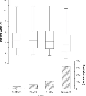
Depths to groundwater ranged between 0.99 and 10.72 m below ground surface for the study period (Fig. 3). Medians of the values decreased, which meant water level rise, by 0.72 m from 4.27 m in March to 3.55 m in August. The rise of the water level coincided with amount of precipitation of the month. Groundwaters generally flow from southwest to
northeast, toward the main stream (oblique to the stream;
see Fig. 1). Hydraulic gradients ranged from 0.083 in the hill area to 0.015 in the central area.
2.3. Auto-Correlation and Cross-Correlation
Although the water level fluctuations are not physically outputs of the aquifer system to rainfall, the cross-correla- tion between the site rainfall and the corresponding water- level variations can give us useful information on patterns of temporal variation of hydrologic process and impulse response characteristics of aquifer systems (Larocque et al.,
Table 1. Well completion data of the six monitoring wells.
Wells GW16 GW10 GW15 GW9 MW13 GW1
Inner diameter (mm) 50.8 50.8 50.8 50.8 50.8 50.8
Screen interval (depth, m) 3.0−9.0 8.3−14.3 5.0−15.5 6.7−17.5 6.1−13.5 7.5−15.0
Well depth (m) 9.0 14.3 15.5 17.5 19.6 15.0
Distancea (m) 10 120 10b 456 568 720
aDistance from the main stream.
bDistance from the subsidiary stream (bottom of the right side of the study area)
Table 2. Hydraulic properties at six selected monitoring wells.
Wells GW16 GW10 GW15 GW9 MW13 GW1
K (cm/sec) 7.50×10⁻³ 5.31×10⁻³ 6.66×10⁻⁴ 2.15×10⁻³ 5.00×10⁻⁴ 5.02×10⁻⁴
Sya (-) 0.03 0.03 0.02 0.03 0.02 0.02
aMean of specific yields estimated from the laboratory experiments and aquifer tests for the fill soils.
Fig. 3. Ranges of depth to water (DTW) from March to August with monthly precipitation.
1998; Lee and Lee, 2000). In this study, both of the time and frequency domain functions, auto-correlation, spectral density, cross-correlation are used to characterize the hydro- geological system.
For a given set of time series xt, the auto-covariance γk and auto-correlation ρk can be calculated as:
(1) (2) where µ is the mean of xt, k is the time lag, and n is the length of the time series. The auto-correlation functions quantify the linear dependency of successive values over a time period (Larocque et al., 1998) and memory effect (Angelini, 1997). If the time series is random, such as rain- fall, the auto-correlation function shows a very quick decrease and reaches a null in a short time lag. However, if the time series has strong inter-dependency and a long memory effect, the auto-correlation function shows a gentle decrease.
The spectral density function in the frequency domain is a Fourier transformation of the auto-correlation function in the time domain. From the spectral density function the periodical characteristic of a time series can be identified:
(3) (4) where f is the frequency, m is the truncation point at which the analysis is carried out, and w(k) is the Tukey filter, which has often been adopted for the analysis of the hydrological series (Mangin, 1984; Padilla and Pulido-Bosch, 1995;
Larocque et al., 1998). The filter overcomes a bias or trun- cation error of spectral density values caused by the finite length of the time series. The regulation time, S(0)/2, obtained from the spectral density function defines the duration of the influence of the input signal and gives an indication of the length of the impulse response of the system (Larocque et al., 1998; Lee and Lee, 2000).
The cross-covariance function between two time series xt and yt is defined as:
(5) where µx and µy are the means of the two time series. For k> 0, the cross-correlation function ρxy is obtained as:
(6) where σx and σy are the standard deviations of the xt and yt, respectively. The cross-correlation function represents the
inter-relationship between the input and output series. If the input stress is a random process such as rainfall, the cross- correlation function is an impulse response function of the aquifer (Padilla and Pulido-Bosch, 1995; Larocque et al., 1998). The delay, which is the time lag between k=0 and the maximum ρxy(k), determines the stress transfer velocity of the system.
2.4. Estimation of Recharge Using Groundwater Level Data Recharge based on the WTF method for unconfined aqui- fers is calculated as (Healy and Cook, 2002):
(7) where Sy is specific yield, h is water-table height, and t is time. The method is best applied over short time periods (hours or a few days) in regions having shallow water tables that show sharp rises and declines (Scanlon et al., 2002).
When delayed drainage occurs, the method would underes- timate the recharge rate (Healy and Cook, 2002).
Moon et al. (2004) suggested a modified WTF method to estimate groundwater recharge as the product of specific yield and the ratio of water-level rise over the cumulative pre- cipitation within the period that caused the water-level rise:
(8) where α is recharge ratio, h is the water-level rise for each precipitation event, and P is the precipitation in each time interval. The modified method produced comparable recharge estimates with those estimated using the baseflow separation method for water-level data of 62 shallow groundwater wells of the national groundwater monitoring stations (Moon et al., 2004). For this comparison study, the modified WTF method was also used.
3. RESULTS AND DISCUSSION 3.1. Water-Level Fluctuation
Time series data of water levels obtained from the six monitoring wells are presented in Figure 4. The fluctuation behaviors caused by the local precipitation were quite dif- ferent among the six wells. Downgradient wells (closer to the stream) showed a rapid rise and decline of water levels in response to the precipitation, while upgradient wells showed slower responses. During the monitoring period of 60 days, it rained over 0.1 mm for 29 days, a characteristic of wet season in the monsoon weather (Lee and Lee, 2000).
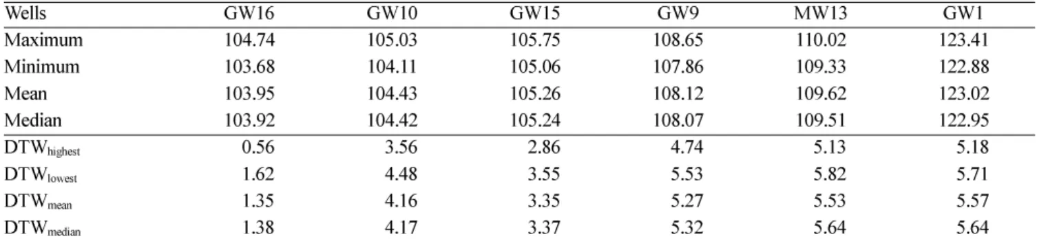
Table 3 shows a summary of the water-level data obtained from the six wells. Water levels ranged between 103.68 and 123.41 m and mean water levels of each well were between 103.95 and 123.02 m. As with topographic elevation, the
γk Cov x( t,xt k+ ) 1
n--- [(xt–µ)(xt k+ –µ)]
t=1 n k–
= = ∑
ρk Cov x( t,xt k+ )
Cov x( t,xt)
--- γγk ----o
= =
S f( ) 2 1 2 w k( )ρkcos 2( πfk)
k=1
∑m
+
= w k( ) 1
2--- 1 cos[ + (πk m⁄ )]
=
γxy( )k Cov x( t,yt k+ ) 1
n--- [(xt–µx)(xt k+ –µy)] t=1
n k–
= = ∑
ρxy( ) γk xy( )k
σxσy
---
=
R Sydh
---dt Sy∆h t ---∆
= =
α h1+ +h2 …+hn
P1+ +P2 …+Pn
---×Sy Σh
ΣP ---×Sy
= =
water levels increased from the stream (GW16) to the hills (GW1). Amplitude of fluctuation during the monitoring period was 0.53−1.06 m. The largest fluctuation occurred at GW16 and the smallest one did at GW1. The fluctuation amplitude appeared partly related to the thickness of the unsaturated zone and the distance to discharge area (main stream). Where the unsaturated zone is thick, the ground- water level changes smoothly (Moon et al., 2004) and
resulting amplitude is small (Fig. 5a). In addition, delayed drainage would cause smoothing water-level change in upgradient area. Quick response and large fluctuation were significant in downgradient area (Fig. 5b). Water levels were shallowest at GW16 [0.56−1.62 m below ground surface (bgs)] and deepest at MW13 (5.13−5.82 m bgs).
Apparently deep groundwater levels at MW13 were due to the relatively thick fill soils in this location (see Fig. 2).
Fig. 4. Groundwater hydrographs of the six monitoring wells, (a) GW1, (b) MW13, (c) GW9, (d) GW15, (e) GW10, and (f) GW16.
Table 3. Summary of the water-level data of the six wells. DTW is depth to water below ground surface. Units are in m.
Wells GW16 GW10 GW15 GW9 MW13 GW1
Maximum 104.74 105.03 105.75 108.65 110.02 123.41
Minimum 103.68 104.11 105.06 107.86 109.33 122.88
Mean 103.95 104.43 105.26 108.12 109.62 123.02
Median 103.92 104.42 105.24 108.07 109.51 122.95
DTWhighest 110.56 113.56 112.86 114.74 115.13 115.18
DTWlowest 111.62 114.48 113.55 115.53 115.82 115.71
DTWmean 111.35 114.16 113.35 115.27 115.53 115.57
DTWmedian 111.38 114.17 113.37 115.32 115.64 115.64
The interpretation of these data is presented in the fol- lowing sections.
3.2. Auto- and Cross-Correlation
Autocorrelation and spectral density functions of the water levels are presented in Figure 6. Autocorrelations were very similar in shapes but two characteristic groups (GW1, MW13; GW16, GW15) can be identified according to decreasing trend. As shown in the groundwater hydrographs (see Fig. 4), one group shows relatively smooth variation pattern and the other shows very steep response pattern.
Two wells (GW9, GW10) showed mixed or intermediate responses. These phenomena can be identified in time lag and regulation time (Table 4) as well. Longer time lag reflects a stronger inter-dependency and a longer memory effect. The regulation time indicates the duration of the influence of the input signal and gives an indication of the length of the impulse response of the aquifer system (Lee and Lee, 2000). Therefore, shorter regulation times of GW15 and GW16, which are proximal to the streams, represented quicker dissipation of input stress (rainfall). Relatively higher values of spectral density of these wells at high fre- quency also support the quick responses and quick dissipa- tion to the stress (see Fig. 4). Interestingly, the autocorrelation function of the site rainfall quickly reaches a null value. This is an indicator of an uncorrelated (ran- dom) characteristic of the hourly rainfall (Angelini, 1997;
Lee and Lee, 2000), which is also identified from much evenly distributed spectral density at high frequencies.
Autocorrelation and spectral density functions of daily averaged water levels are shown in Figure 7. Like the results of the hourly based time series analyses, the two groups (GW1, MW13; GW15, GW16) can also be identi- fied from the decreasing trend of autocorrelation and mag- nitude of spectral density. Most interestingly, both the precipitation and stream levels showed much different behaviors from the other wells. The auto-correlation func- tions of the rainfall quickly reach a null value. The spectral density function shows oscillatory behavior over all fre- quencies. These are all indicators of a random characteristic (weakly inter-dependent) of the daily rainfall (Lee and Lee, 2000). The stream levels showed similar behavior, which indicates that it has very close correlation with the site rain- fall (r=0.869). As expected, significantly shorter time lag and regulation time of the stream level rather than the groundwater levels also showed its quick response and quick dissipation of the stress (see Table 4).
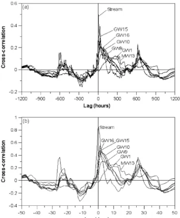
Cross-correlation between the site rainfall and the groundwater levels are presented in Figure 8 and Table 5.
Correlation and time delay showed a systematic change with respect to thickness of the unsaturated zone and dis- tance to the main stream. The stream level showed highest correlation with rainfall at no substantial lag time (0 day;
Fig. 9). Secondly highest correlations were found at GW16 (r=0.552) and GW15 (r=0.485) wells with a lag time of 1 day. These wells are most proximal to the streams and the
Fig. 5. Relationships between amplitude of water-level fluctuation and (a) mean thickness of unsaturated zone and (b) distance to the main stream. Data of GW15, very proximal to the subsidiary stream, was omitted for the plots.
Table 4. Results of the auto-correlation analyses with the hourly and daily basis water levels of the six wells.
Wells GW16 GW10 GW15 GW9 MW13 GW1 Stream Rain
Time lag (hr) 301.4(12.6)a 439.8(18.3) 267.2(11.1) 431.4(18.0) 446.9(18.6) 411.5(17.1) 198.2(8.3) 39.8(1.7) Regulation time (hr) 154.3(6.4)a 249.8(10.4) 135.2(5.6) 249.4(10.4) 288.6(12.0) 274.6(11.4) 52.1(2.2) 3.9(0.2)
Time lag (days) 13.9 19.2 11.6 18.6 18.8 17.5 4.8 3.9
Regulation time (days) 10.5 12.6 8.1 12.5 13.9 13.5 3.4 2.4
aParenthesis indicates time in days
unsaturated zones around the wells are thinnest. So signal of the input stress (rainfall) was least attenuated during per- colation of the soil zone resulting in high correlation with the rainfall and large amplitude of water-level fluctuation.
This interpretation is based on the assumption that ground- water recharge mostly occurs by vertical percolation of the site rainfall and delayed drainage can be neglected. Water levels of MW13 and GW1 wells showed lowest correla- tions with the rainfall (r=0.277 and 0.306) at much larger lag times (7 and 3 days, respectively), which indicated larger attenuation of the input stress due to longer percolation length.
Between hourly and daily-based correlation analyses, time delays of the hourly data were generally shorter. This means that the daily water levels may conceal hydrologic information of the hourly input stress and response. Dis- tinctly, maximum correlations greatly increased in the daily analyses. Daily lumped rainfall showed a much higher cor- relation with the groundwater levels than hourly separate rainfall did. This means that it takes a few hours or longer for rainwater to reach the water table.
3.3. Recharge Estimates
Recharge ratios at the monitoring wells were estimated
Fig. 6. Autocorrelation and spectral density functions for the water levels of the six monitoring wells, stream level, and local precipitation (truncation points=1,200 hours).
Fig. 7. Autocorrelation and spectral density functions for daily averaged water levels of the six monitoring wells, stream level, and local precipitation (truncation points=50 days).
Fig. 8. Cross-correlation between hourly- and daily-basis water levels and rainfall.
using the modified WTF method (Moon et al., 2004) in consideration of the time delays. First, water-level rise due to event rainfall was calculated (Fig. 10). Any noticeable water-level rise in case of no rainfall indicated existence of delayed drainage by preceding rainfall or horizontal com- ponent of groundwater recharge. In this case, meaningful water-level rises were observed at minimum rainfalls of 5−10 mm. The water-level rises versus event rainfall were fitted with linear equations but they yielded a wide range of coefficients of determination (r2=0.19−0.93).
As expected, the same amount of precipitation did not produce the same amplitude of water-level rise. Water-level rises due to specific amount of rainfall were largest at GW16
Fig. 9. Hydrograph of the main stream with rainfall.
Fig. 10. Water-level rises due to event rainfall at the six monitoring wells.
while those were smallest at GW1. At MW13, the water- level rises were relatively small and linearity between the water-level rise and the rainfall was poorest. The fact is highly correlated with larger attenuation of the input stress through the thickest unsaturated zone, which amplified the non-linearity (Kim, 2001). This is also supported by the lowest correlation between rainfall and water level, and largest time delay (see Table 5). Excellent linearity between water-level rises and site rainfall was observed at GW15 (r2=0.87) and GW16 (r2=0.93) wells, which were located in the downgradient area.
To obtain the recharge ratios, the ratios of the rise in groundwater level and the cumulative rainfall during the rainy period were calculated (Table 6). Subsequently, the recharge ratios were computed using these ratios and the specific yields (see Table 2). As expected, the same amount of the cumulative precipitation produced a wide range of water-level rises for different monitoring locations due to different hydrogeological conditions such as the thickness of the unsaturated zone and the distance to discharge area.
Estimates of the recharge ratios based on the modified WTF method ranged from 2.5 to 20.1%. The largest value of the recharge ratio was obtained at GW16, the most downgra- dient well while the lowest value was estimated at GW1, the most upgradient well. Although the spatial extent of the monitoring area is only 0.256 km2, the estimated recharge ratios are very different by up to a factor of 8.
Meanwhile Korea Water Resources Corperation (KOWACO) (2005) estimated an average recharge ratio of 12.7% for the whole basin area (867 km2) including the study area based on the water budget analysis and the groundwater hydro- graphs of the national groundwater monitoring stations.
Simple mean of the six recharge estimates of this study is 9.6%, which is not quite different from that of KOWACO.
However, considering the great difference of the recharge ratios according to the monitoring locations even in the small area, it is very important to choose appropriate loca-
tion of groundwater monitoring. For example, the monitor- ing location should not be very close to streams but the subsurface geology of the monitoring well should represent enough that for the whole area of interest.
4. SUMMARY AND LIMITATIONS
Groundwater recharge is an important factor in planning sustainable groundwater development. In this study, recharge ratios were estimated based on the modified water-table fluctuation method using the water level data from a small area. Although the study area is very small, the fluctuation behaviors of groundwater levels in response to rainfall were very different depending on the thickness of the unsaturated zone and the distance from the monitoring well to the main stream. Where the unsaturated zone is thick, the ground- water level in response to rainfall changes smoothly and resulting amplitude is small. Where the distance to the stream is short, the hydrographs showed a quick response and large fluctuation. According to the monitoring loca- tions, the recharge estimates showed a very wide variation between 2.5 and 20.1%. Compared with 12.7% estimated by other study mainly based on the water budget analyses, the recharge ratios were underestimated in upgradient area while they were overestimated in downgradient area. Therefore, water-level monitoring locations should be carefully selected, to reflect the study area such as surface conditions, subsur- face geology, and hydrologic boundary.
However, some limitations were left unexplained in this study. First, effects of moisture conditions of the surface and subsurface soils were not considered. As known, amounts of runoff, infiltration, and rainfall trapped in the unsaturated zone are dependent on the moisture conditions. Conse- quently, the same amount of rainfall may not produce same water-level rises. This can be partly perceived in that same amount of rainfalls produced very different water-level rises at the same monitoring well at different times (see Fig. 10).
Table 6. Cumulative precipitation, water-level rise and recharge ratios at six selected monitoring wells.
Wells GW16 GW10 GW15 GW9 MW13 GW1
ΣP (mm) 613 613 613 613 613 613
ΣH (mm) 4,114 2,686 2,880 1,533 1,557 762
ΣH/ΣP 6.71 4.38 4.70 2.50 2.54 1.24
Recharge ratio (%) 20.1 13.1 9.4 7.5 5.1 2.5
Table 5. Time delays and maximum correlation obtained from hourly and daily basis cross-correlation analyses.
Wells GW16 GW10 GW15 GW9 MW13 GW1 Stream
Time delay (hours) 29(1.2)a 39(1.6) 1(0.04) 41(1.7) 159(6.6) 46(1.9) 3(0.13)
Maximum correlation 0.290 0.206 0.325 0.215 0.129 0.140 0.501
Time delay (days) 1 2 1 2 7 3 0
Maximum correlation 0.552 0.453 0.485 0.466 0.277 0.306 0.869
a Parenthesis indicates time in days
Second, as noted by Moon et al. (2004), the recharge ratios in this study were estimated using the groundwater hydro- graphs for the wet season in the country and so they may represent upper limits for the study area. Consequently, a same kind of analyses should be conducted for the dry sea- son (November-February). In addition, effects of delayed drainage and horizontal recharge from surrounding or remote area were not addressed. The stream-level fluctuation can affect the water level of neighboring groundwater wells, which can be quantified if the stream bed conductance is known. They deserve a further study.
ACKNOWLEDGEMENT: The authors wish to thank Prof. Jae- Young Yu at Kangwon National University and two anonymous reviewers for their critical comments improving the initial manuscript.
REFERENCES
Angelini, P., 1997, Correlation and spectral analysis of two hydro- geological systems in Central Italy. Hydrological Sciences Jour- nal, 42, 425−439.
Beekman, H.E. and Xu, Y., 2003, Review of groundwater recharge estimation in arid and semi-arid Southern Africa. In: Xu, Y. and Beekman, H.E. (eds.), Groundwater Recharge Estimation in South Africa. UNESCO IHP Series No. 64, p. 3−18.
de Vries, J.J. and Simmers, I., 2002, Groundwater recharge: an over- view of processes and challenges. Hydrogeology Journal, 10, 5−17.
Healy, R.W. and Cook, P.G., 2002, Using groundwater levels to esti- mate recharge. Hydrogeology Journal, 10, 91−109.
Kim, T.H., 2001, An Alternative Framework for Analyzing Hydrau- lic Information of the Groundwater Flow System. Ph.D. thesis, Seoul National University, Seoul, 177 p.
KOWACO (Korea Water Resources Corp.), 2005, A Basic Plan on Management of Groundwater Resources in Kangwon Province.
KOWACO, Daejon. (unpublished)
Larocque, M., Mangin, A., Razack, M. and Banton, O., 1998, Con- tribution of correlation and spectral analyses to the regional study of a karst aquifer (Charente, France). Journal of Hydrology, 205, 217−231.
Lee, J.Y., 1998, Use of Field Observations to Characterize a Frac- tured Porous Aquifer System in Won-Ju, Korea. M.S. thesis, Seoul National University, Seoul, 114 p.
Lee, J.Y. and Lee, K.K., 2000, Use of hydrologic time series data for identification of recharge mechanism in a fractured bedrock aqui- fer system. Journal of Hydrology, 229, 190−201.
Lee, J.Y., Choi, M.J., Kim, Y.Y. and Lee, K.K., 2005, Evaluation of hydrologic data obtained from a local groundwater monitoring net- work a metropolitan city, Korea. Hydrological Processes, 19, 2525-2537.
Lerner, D.N., 2003, Surface water-groundwater interactions in the context of groundwater resources. In: Xu, Y. and Beekman, H.E.
(eds.), Groundwater Recharge Estimation in South Africa. UNESCO IHP Series No. 64, p. 91−107.
Mangin, A., 1984, Pour une meilleure connaissance des systemes hydrologiques a partir des analyses correlatoire et spectrale. Jour- nal of Hydrology, 67, 25−43.
Moon, S.K., Woo, N.C. and Lee, K.S., 2004, Statistical analysis of hydrograph and water-table fluctuation to estimate groundwater recharge. Journal of Hydrology, 292, 198−209.
Padilla, A. and Pulido-Bosch, A., 1995, Study of hydrographs of karstic aquifers by means of correlation and cross-spectral anal- ysis. Journal of Hydrology, 168, 73−89.
Park, B.K., Chang, H.W. and Woo, Y.K., 1989, Geologic Report of the Wonju Sheet. KIER (Korea Institute of Energy and Resources), Daejon, 6 p.
Scanlon, B.R. and Cook, P.G., 2002, Theme issue on groundwater recharge. Hydrogeology Journal, 10, 3−4.
Scanlon, B.R., Healy, R.W. and Cook, P.G., 2002, Choosing appro- priate techniques for quantifying groundwater recharge. Hydro- geology Journal, 10, 18−39.
Wilson, L.G. and de Cook, K.J., 1968, Field observations on changes in the subsurface water regime during influent seepage in the Santa Cruz River. Water Resources Research, 4, 1219−1234.
Won, J.H., Kim, J.W., Koh, G.W. and Lee, J.Y., 2005, Evaluation of hydrogeological characteristics in Jeju Island, Korea. Geosciences Journal, 9, 33−46.
Manuscript received February 17, 2005 Manuscript accepted June 15, 2005