• 검색 결과가 없습니다.

A Study on a New Approach to Robust Control and Torque Control Response Analysis of Manufacturing robot Based on Monitoring Simulator for Smart Factory

N/A
N/A
Protected

Academic year: 2021

Share "A Study on a New Approach to Robust Control and Torque Control Response Analysis of Manufacturing robot Based on Monitoring Simulator for Smart Factory"

Copied!
13
0
0

로드 중.... (전체 텍스트 보기)

전체 글

(1)

A Study on a New Approach to Robust Control and Torque Control Response Analysis of Manufacturing robot

Based on Monitoring Simulator for Smart Factory

Hee-Jin Kim 1 , Dong-Ho Kim 1 , Gi-Won Jang 1 , Byeong-Hwa Gu 1 , Sung-Hyun Han 2

<Abstract>

This study proposes a new approach to implimentation of robust control and torque control response analysis based on monitoring simulator for smart factory. According to the physical properties of a flexible manipulator, a two time-scale approach, namely, singular perturbation ap proach, is further utilized for thorough analysis and general controller design. It is shown that asymptotic motional tracking can be effectively achieved, whereas the force regulation errors can be made arbitrarily small.

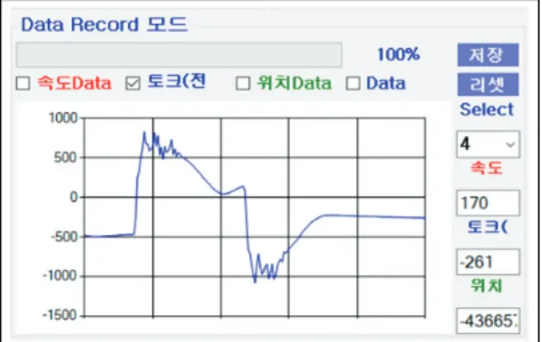
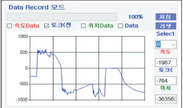
For demonstration of the proposed technology performance, experiments of a eight joint flexible manipulator are performed for the proposed control method, and the reliability of proposed control results are illustrated based on monitoring simulator.

Keywords : Robust Control, Torque Control, Response Analysis, Monitoring Simulator, Smart Factory

1 Corresponding Author, Department of Mechanical Engineering, Graduate School, Kyungnam Univ.

E-mail: [email protected]

2 Professor, Department of Mechanical Engineering, Kyungnam Univ.

E-mail: [email protected]

(2)

1. Introduction

In the recent decade, increasing attention has been given to the tracking control of robot manipulators. Tracking control is needed to make each joint track a desired trajectory. A lot of research has dealt with the tracking control problem: were based on VSS (variable structure system) theory, on adaptive theory, and on Fuzzy logic. Robots have to face many uncertainties in their dynamics, in particular structured uncertainty, such as payload parameter, and unstructured one, such as friction and disturbance. It is difficult to obtain the desired control performance when the control algorithm is only based on the robot dynamic model. To overcome these difficulties, in this paper we propose the robust control schemes which utilize a neural network as a compensator for any constrints.[1]

In the literatures, many fundamental issues on this regard have been extensively studied, such as impact analysis and contact force regulation, compliant force regulation, and force/position control during constrained motion. In [2], a standard approach for constrained manipulation have been developed, in which a systematic way is employed to reduce the system dynamics into lower-order ones and then a nonlinear feedback controller is designed to deal with the constrained system. Other controller designs based on the theory of variable structure systems [3], learning algorithm [5],

and parallel approach [3] have also been developed in the past. Jean and Fu [4]

proposed an adaptive hybrid control scheme for the constrained robots based on both Lagrange and Newton-Euler dynamics formulations, and Stepanenko and Su [4]

developed a controller which can adaptively tune the gains of the variable structure scheme[2]. This basic control system enables a manipulator to perform simple positioning tasks such as in the pick-and-place operation. However, joint control- lers are severely limited in precise tracking of fast trajectories and sustaining desirable dynamic performance for variations of payload and parameter uncertainties (R. Ortega et al., 1989; P. Tomei, 1991). In many servo control applications the linear control scheme proves unsatisfactory, therefore, a need for nonlinear techniques is increasing.[3]

For industrial applications, many extensive studies of flexible manipulators have been carried out. Dynamic models of multilink flexible manipulators are completely derived by Book and Luca and Siciliano [5]. Many nonlinear control schemes such as those using computed torque, inverse dynamics, and feedback linearization, 35], have all been thoroughly developed for multilink flexible manipulators in the past decades. Extensive experimental studies of flexible manipulators have been demonstrated in [4].

In this paper, the 8-link dual-arm robot

has been built up to demonstrate the

performance of the proposed method, and

(3)

experimental results have validated the effectiveness of the proposed control scheme.

2. Robotic Manipulator Dynamics

This study consider the flexible manipulator whose end-effector is in contact with the environment modeled as frictionless surface.

In the following derivation, we will use the subscripts and to denote the rigid-mode part and flexible-mode part, respectively. The dynamics of the constrained flexible manipulator can be derived by using the Lagrangian formulation via the assumed mode method which appear in the following form(5):

   



 



 

   



 





 

 

  

   

 

(1)

with

   ′     (2)

where    

′ ,    

′ , ,  ∈  ,

∈ 

,   , and ′  with      . For convenience, we first define the inverse of the inertia matrix as:

   



     

   



  (3)

so that (1) becomes

                  (4)

                  (5)

where

   



    

   



 

   



 

 

    

   



 

 

 

 

   

   



 

As a matter of fact, when a manipulator is constrained by its environment, it is more convenient and realistic to use the coordinates in Cartesian space (i.e. task space) rather than the joint configuration space. Thus, in the following derivation, we will derive the equations of motion in Cartesian coordinates. Therefore, let the position of the end-effector be described as

    , where  →  ,

      . If we take the first and the second time derivative of , we will then have the relations of velocities and accelerations in joint space and in Cartesian space as follows[6][7]:

       (6)

             (7)

(4)

where    

 

,    

 

. Without loss of generality, we have assumed that the flexible manipulator is non-redundant with respect to the rigid part, which implies  is invertible for almost all  ∈ , except maybe when

is at certain configurations. For simplicity, in the rest of this paper, we will assume that the manipulator will be operated solely in the region where  is uniformly invertible, which is doable if the desired motion trajectory can be somewhat carefully chosen.

Therefore, we can obtain[7].

  



 

 

 

  



 





  



 

 



 

 

 

 



 

  



 

 (8)



 



 





  



 





  



 

 



 

 

 

 



 

  



 

 (9)

where

             

        

             

                 

       

      

    

    

        

       

   

  

 

Now, we are ready to formulate the above dynamic model into a singular perturbation form via the definitions    and where is a common factor extracted from each entry of the matrix , assumed to be small enough. Further, we define the variables  and  as equation(8) and (9), respectively, as follows:

  



 

  

 

 

 

 

  

 (10)

  



    

  

 

 

 

 

  

(11)

which amounts to the singular perturbation model of the flexible manipulator system.

One should note that the matrix plays the role of a constant stiffness matrix and, hence, the overall system becomes stiffer if is uniformly larger or, equivalently, is made smaller. According to the singular perturbation theory, the model obtained above will tend to a rigid model provided the system rigidity gradually diminishes. It can be shown that as  →  , (10) becomes the model of a rigid manipulator, i.e., as

 →  , one can obtain(10)

   

                     (12)

and, hence, the rigid manipulator model can

be readily derived as:

(5)

   

           

         

            

(13)

where we have used the relation  

         , and all the variables with overbar are simply to denote those in the situation where    .

For deriving the fast subsystem, we let the fast time-scale be    and redefine the fast variables       and    . Thus, the fast subsystem can be derived as[9]:

 

 

 

   

 

  



 

 

   

 



     (14)

or equivalently,

 

      (15)

Note tat  is the control input to the fast subsystem. As opposed to the objective of designing the slow mode control, the fast mode control  is devised to make the set point    uniformly exponentially stable.

Hereafter, we will separately design the control inputs  and  corresponding to the slow and the fast subsystems, respectively.

Next, due to the existing constraints, we will reduce the set of original equations of motion into a more realistic form. First, we divide the state , or equivalently  , in the slow subsystem into two parts, namely,

and  , where  ∈  and  ∈     and assume the constraint can be reexpressed as:

             (16)

where is a nonlinear map form    to

. Furthermore, we can obtain the velocity and acceleration relations between  and

as:

          

        

(17)

where     

 

is assumed to be of full rank. Then we rewrite the state-space equations into the differential equations in terms of the Cartesian state, , by premultiplying the equations by

       and then using the following relatio[12].

   



 

   

 

 

 

     

so that the resulting equations become:

 

 



 

   

 



 

  

 



 



 



 

 

 

  

 

  

  

(18)

For convenience of analysis, we can further

partition the matrices and rewrite the above

equations into the following form:

(6)

 

 

   

   

 

 

 

 

 

  



   

 

   

 

  

 

(19)

Clearly,

       is symmetric and positive definite. Now, if equation(17) is used to replace  ,  ,  in (19), and then premultiply the upper part of equation (19) by

and add the results to its lower part, then the following equations are obtained[12].

                 (20)

                     (21)

where

         

                  

             

               

            

Thus, we can refer to the equations (20) and (21) as force part and motion part, respec- tively. In the next section, we will design the controller based on the reduced slow-subsystem[11].

3. Control Algorithm

Our objective is to design a hybrid controller to achieve asymptotic tracking of both unconstrained coordinates  and constrained forces , i.e., to yield

 →    and  →    as  → ∞

Before we proceed to present the controller design, we will summarize some useful dynamical properties of the flexible manipulators in the following proposition.

Proposition 3.1: For the constrained flexible manipulator described in the previous section, the following properties will hold[14).

1)  is symmetric and positive definite.

2) By a proper choice of      to define

  , the matrix     is skew-sym- metric.

3) There exist some constant vectors  

and

 such that

              (22)

                  

     

(23)

where  and  are known functions of their arguments.

Now, we are ready to introduce process of

designing a controller for the manipulator

(7)

system in the following.

We first define the auxiliary signal as

       (24)

where        is the tracking error and

is some positive constant.

Let the control laws be designed as[15]:

          (25)

              (26)

for (20) and (21), respectively, where  

            and  , denote the estimates of system parameters    

and the measurement of contact force . Let the parameter adaptation law be devised as:

 

 

  

               (27)

where             and is some positive constant.

Accordingly, the error dynamics can be obtained by the following derivation with the help of equation (10) and equation (11), i.e.,

                   

                 

                      

                         

(28)

               

                 

                  

        

                

                 

(29)

where     is the parameter estimation error and      is force tracking error.[15]

If we choose the Lyapunov function candidate  as:

   

      

     (30)

and take its time derivative along the trajectories of (28) and (29), then, by virtue of Proposition, we obtain[11)

            

           

                                                            

  ∥  ∥  

  ∥  ≤        

(31)

where       is some positive constant,      

  ∥  , and  is a

(8)

continuous function of which vanishes only at    Therefore, we can guarantee that and will converge to a residual set with size    , and so are      . IN the following, we will show that is also a bounded signal. Consider the closed-loop dynamical equation (28), where  can be represented as

                     (32)

We then apply (32) to (29) to obtain

                                

(33)

Assume that ∥    ∥ ≤  for some constant

 which denotes the possible bound on the force measurements error, the from equation (29), (33) we can obtain

   ∥       (34)

   ∥       (35)

with the constant satisfying

  ∥

                      

In (35), we have theoretically derived the relations between the force tracking and the force measurement error. It is therefore obvious that the force tracking error can be

made arbitrarily small by enlarging  if precise force measurement can be obtained.

We first rewrite equation (15) in the fast time scale as follows:

 

         (36)

Since our control objective is to regulate the fast state , here we design a robust regu- lator. For the full-order system being dominated by the slow subsystem, a state regulator must be devised to force  →  as fast as possible. Within the boundary layer, the system matrices and can be substituted by   ∆  and   ∆  , respectively, where  and  are nominal matrices with known elements plus the known bounds on ∥ ∆  ∥ and ∥ ∆  ∥ . And, we further design a dynamic feedback controller as follows[13]:

 



        (37)

where the matrices and will be determined later, whereby the closed-loop system consisting of (36) and (37) becomes

 

       (38)

where         

 

 

 

   , and  

 

 

∆  ∆ 

  . The following theorem provides

(9)

a condition under which the above design of the fast-subsystem controller may give the desirable result.

If  and  are chosen such that A is Hurwitz and if there exist matrices   satisfying

     (39)

and min     ∥  ∥ , where ∥≤  , then it is guaranteed that ∥∥→

exponentially[12].

Proof: Let the Lyapunov function candidate

be

 

    (40)

and take the fast time derivative of  as follows[14]:

 

 

  

        

       

≤   min   ∥∥  ∥∥∥  ∥∥∥     min     ∥∥∥  ∥∥∥ ≤     

where  is some positive constant and 

is a continuous function which vanishes only at    . Thus, through a Lyapunov theor- em. this theorem can thus be concluded.

This property will be useful in our later derivation of a composite controller[15].

4. Performance Test and Results

4.1 Simulation and Results

The constrained surface, which is made of rigid arm, at the location. The desired motion trajectory is taken to be the form of a fifth-order polynomial trajectory   , where

  

             

and   sec is the expected duration of the motion. The desired contact force is The gain     and  are 5, 12, and 18, respectively. The results are plotted in Fig.(1)-Fig.(6), in which Fig.1 is tracking error of tip position and Fig.2 represents tracking error of contact force. Fig.3 is vibration response mode of link 1 and Fig.4 shows vibration response mode of link 2. Fig.5 is vibration response mode of link 3 and Fig.6 represents vibration response mode of link 4.

Fig. 1 Tracking Error of Tip Position

(10)

Fig. 2 Tracking Error of contact Force

Fig. 3 Vibration Response Mode of Link 1

Fig. 4 Vibration Response Mode of Link 2

Fig. 5 Vibration Response Mode of Link 3

Fig. 6 Vibration Response Mode of Link 4

4.2 Experiment and Results

The reliability of control performance had been verified by experiments for articulated robot with 8 joints. The 8-link flexible manipulator is a planar arm with eight revolute joints which are horizontal type structure.

The first link is driven by a D.C. motor

with ratio 120:1 and the second link is

driven by a D.C. Brushless motor with gear

(11)

ratio 100:1. In addition, the hub of the second joint of the manipulator is airjetted in order to counteract the gravity. The

mathematical model of this flexible manipulator is derived based on the so-called assumed mode method, and the vibration modes.

Fig. 10 The torque Control Response of Joint 3

Fig. 11 The torque Control Response of Joint 4

Fig. 12 The torque Control Response of Joint 5 Fig. 7 Experimental Set-up

Fig. 8 The torque Control Response of Joint 1

Fig. 9 The torque Control Response of Joint 2

(12)

Fig. 13 The torque Control Response of Joint 6

Fig. 14 The torque Control Response of Joint 7

Fig. 15 The torque Control Response of Joint 8

The Fig 7 shows the experiment set-up.

The Fig. 8 represents the torque control response of Joint 1 of a horizontal type robot manipulator with eight joints, and the Fig. 9

shows the torque control response of Joint 2.

The Fig. 10 represents torque control response of Joint 3, and the Fig. 11 shows the torque Control Response of Joint 4. The Fig. 12 shows torque control response of Joint 4, and Fig. 13 shows the torque control response of Joint 6. The Fig. 14 shows the torque control Response of Joint 7. The Fig. 10 shows the torque control response of Joint 8.

5. Conclusions

In this study, we proposes a new approach to robust control technology, and torque control response analysis based on monitoring simulator for a horizontal type robot manipulator with eight joints. In this paper, an robust control algorithm in cartesian space proposed based on nonlinear control method including with singular perturbation. The experiments of horizontal type dual arm robot with eight joints has been set up to illustrate the performance and reliability of the proposed robust control and monitoring simulato.r. The verification of proposed method was proved by simulatio0n and experiments.

Acknowledgement

This study was supported by Industrial Technology Innovation Project (Project Number.

20005020).

(13)

References

[1] H.J. Kim, G.W. Jang, D.H. Kim and S.H. Han,

“A Study on Track Record and Trajectory Control of Robot Manipulator with Eight Joints Based on Monitoring Simulator for Smart Factory”, KSIC.2020.23.4 pp. 549-558.

[2] H.J. Kim, D.H. Kim, K.J. Jung and S.H. Han,

“A Study on Performance Analysis of Artic- ulated Robot System for Smart Factory Based on Monitoring Simulator”, KSIC.2020.23.6 pp.

889-896.

[3] S.H. Kim, D. B. Kim, H.J. kim, O.D. Im and S.H. Han, “A Study on Real Time Control of Moving Stuff Action Through Iterative Learning for Mobile-Manipulator System”, KSIC.2019.22.4 pp. 415-425.

[4] W.S. Lee, M.S. Kim, H.Y. Bae, Y.K. Jung, Y.H. Jung, G.S. Shin, I.M. Park and S.H. Han,

“A Study on Stable Motion Control of Humanoid Robot with 24 Joints Based on Voice Command”, KSIC.2018.21.1 pp. 17-27.

[5] H.S. Sim, H.Y. Bae, D.B. Kim and S.H. Han,

“A Study on Flexible Control and Design of Robot Hand Fingers with Eight Axes for Smart Factory”, KSIC.2018.21.4 pp. 183-189.

[6] Book, W. J., “Recursive Lagrangian dynamics of flectible manipulator arms,” Int. J. of Robot.

Res., vol. 3, no. 3, Fall, pp. 87-101, 1984.

[7] Carusone, J., K. S. Buchan, and G. M. T.

D’Eleuterio, “Experiments in end-effector tracking control for struc-turally flexible space manipulators,” IEEE Trans. Robot. Automat., vol. 9, no. 5, pp. 553-560, 1993.

[8] Chiaverini, S. and L. Sciavicco, “The parallel approach to force/position control of robotic manipulator,” IEEE Trans. Robot. Automat., vol.

9, no. 4, pp. 361-373, Aug. 1993.

[9] Jean, J.-H. and L.-C. Fu, “Adaptive hybrid control strategies for constrained robots,” IEEE Trans. Robot. Automat., vol. 35, no. 4, pp.

598-603, April 1993.

[10] Jeon, D. and M. Tomizuka, “Learning hybrid force and position control of robot manipulators,” IEEE Trans. Robot. Automat., vol. 9, no. 4, pp. 423-431, Aug. 1993.

[11] Lew, J. Y. and W. J. Book, “Hybrid control of flexible manipulators with multiple contact,”

Proc. IEEE Conf. Robot. Automat., pp. 242- 247, 1993.

[12] Lewis, F. L. and M. Vandegrift, “Flexible robot arm control by a feedback linearization/singular perturbation ap-proach,”

Proc. IEEE Conf. Robot. Automat., pp.

729-736, 1993.

[13] Luca, D. A. and B. Siciliano, “Closed-form dynamic model of planar multilink lightweight robots,” IEEE Trans. Syst. Man Cybernetics, vol. 21, no. 4, pp. 826-839, July/August 1991.

[14] Matsuno, F. and K. Yamamoto, “Dynamic hybrid posi-tion/force control of a flexible manipulator,” Proc. IEEE Conf. Robot.

Automat., pp. 462-467, 1993.

[15] McClamroch, N. H. and D. Wang, “Feedback stabiliza-tion and tracking of constrained robots,” IEEE Trans. Automat. Contr., vol. 33, no/ 5, pp. 419-426, May 1988.

[16] Paden, B., D. Chen, R. Ledesma, and E. Bayo,

“Expo-nentially stable tracking control for multijoint flexible-link manipulators,” ASME J.

Dyn. Syst. Meas. Contr., vol. 115, pp, 53-59, Mar. 1993.

(Manuscript received July 12, 2021;

revised August 04, 2021; accepted August 06, 2021)

수치

Fig.  1  Tracking  Error  of  Tip  Position
Fig.  2  Tracking  Error  of  contact  Force
Fig.  12  The  torque  Control  Response  of  Joint  5Fig.  7  Experimental  Set-up
Fig.  15  The  torque  Control  Response  of  Joint  8

참조

관련 문서

Laser cutting process is one of flexible rapid manufacturing technologies with various advantages including a high cutting speed, manufacturing of parts with

근래에 연구되는 격자형 모델은 각 경계범위에서 각기 다른 변수의 영향을 정확 하게 산출하지 못하고 있으나 , 수용모델링을 병행하는 경우 높은 정확도를 추정할

 A series of systems for configuring alarm and control functions by monitoring the states of main engine, generator, and auxiliary equipment, for securing the safety

The torque analysis was performed acting on the joint of robot by modeling the kinematics and dynamics of the robot.. Load torque of the joint

Wang, “Medium access control with a dynamic duty cycle for sensor networks,” IEEE Wireless Communications and Networking Conference, vol.. Dubendorfer,

Many studies using the assumed mode method have been found for the free vibration analysis of stiffened plate with known elastic boundary conditions.. However

In addition, I carried out a comparative analysis of Sekwang New Beyer and Piano Adventures for composition, features, fundamental position, the form of

In order to derive a new fuzzy controller, a fixed design-parameter fuzzy PID controller was surveyed in view of deriving a control law based on the