IMPLEMENTATION OF VELOCITY SLIP MODELS IN A FINITE ELEMENT NUMERICAL CODE FOR MICROSCALE FLUID SIMULATIONS
A.D. Hoang1 and R.S. Myong*2
속도 슬립모델 적용을 통한 마이크로 유체 시뮬레이션용 FEM 수치 코드 개발
A.D. Hoang,1 명 노 신*2
The slip effect from the molecular interaction between fluid particles and solid surface atoms plays a key role in microscale fluid transport and heat transfer since the relative importance of surface forces increases as the size of the system decreases to the microscale. There exist two models to describe the slip effect: the Maxwell slip model in which the slip correction is made on the basis of the degree of shear stress near the wall surface and the Langmuir slip model based on a theory of adsorption of gases on solids. In this study, as the first step towards developing a general purpose numerical code of the compressible Navier-Stokes equations for computational simulations of microscale fluid flow and heat transfer, two slip models are implemented into a finite element numerical code of a simplified equation. In addition, a pressure-driven gas flow in a microchannel is investigated by the numerical code in order to validate numerical results.
Key Words : Microscale Gases, Slip Models, Finite Element Method
접수일: 2009년 4월 29일, 수정일: 2009년 6월 16일, 게재확정일: 2009년 6월 19일.
1 경상대학교 대학원 기계항공공학부 항공우주공학전공 2 종신회원, 경상대학교 기계항공공학부 및 항공기부품기술연구소
* Corresponding author, E-mail: [email protected]
1. INTRODUCTION
The theoretical study of nonlinear gas transport in microsystems[1-4] has been considered very challenging owing to the complexity of the physical mechanisms associated with these systems. There exist important issues such as the formulation of high-order governing equations capable of describing fluid flows far away from thermal equilibrium and the development of theoretical models taking into account the true nature of gas-surface molecular interactions. Owing to the relative importance of surface forces in microsystems, the slip effect from the molecular interaction between fluid particles and solid surface atoms plays a non-trivial role in microscale fluid
transport and heat transfer. There exist two models to describe the slip effect: the Maxwell slip model[5] in which the slip correction is made on the basis of the degree of shear stress near the wall surface and the Langmuir slip model[2-4] based on the theory of adsorption of gases on solids.
Recently, there have been numerous works that have investigated microscale fluid flows and heat transfer. For example, several theoretical studies[3,4,6], experimental works[7,8], and a numerical investigation[9] have been conducted on internal flow in a microchannel. However, there exists a numerical difficulty arising from the accommodation coefficient of the conventional Maxwell slip model in the mathematical sense. The expression by the Maxwell slip model is not well-defined mathematically in the limit of vanishing diffusive reflection and, depending on situations, the value of slip is not bounded, which can cause severe problems in the numerical implementation of the model. For example, it was reported that the Maxwell slip model can cause the reversal of slip velocity and an overshoot of slip velocity near the
reattachment point in the study of modeling separation[10].
Furthermore, it can be shown by a simple analysis that in order to ensure the numerical stability for no change in the sign of vorticity at the wall the Knudsen number should be less than the size of the grid, restricting the range of the model significantly, especially if the grid size is refined near the wall. To deal with some of these difficulties, several studies[11-15] based on the Langmuir slip model have been conducted recently; for example, an efficient compressible pressure correction algorithm[11-13].
In this study, as a first step towards developing a general purpose numerical code of compressible Navier- Stokes equations (and conservation laws with new nonlinear constitutive relations[16]) for computational simulations of microscale fluid flow and heat transfer, two slip models are implemented in a finite element numerical code of a simplified equation. Since the nonlinearity observed in constitutive relations of microscale gases is very similar to the generalized Newtonian fluids, the same numerical scheme developed for generalized Newtonian fluids, which is the finite element method[17] in most cases, is chosen as the basic numerical scheme for the simulation of microscale gas flows. In order to validate numerical predictions, a pressure-driven gas flow in a microchannel is investigated.
2. ANALYSIS
2.1 FORMULATION BASED ON THE NAVIER-STOKES
EQUATIONS WITHOUT CONVECTIVE TERMS
In low speed microscale gas flow, the slip effect from the gas-surface molecular interaction remains dominant, while the non-Newtonian effect in the bulk region becomes negligible. Therefore, the Navier-Stokes equations with an appropriate slip boundary condition can be applied to the analysis of the flow. In addition, nonlinear convective terms may be neglected in the case of a very long microchannel. Furthermore, variations in the direction of the width in microchannels can be neglected for microchannels with high aspect ratios. Then, the governing equation derived from the Navier-Stokes equations can be written, in the non-dimensional form, as
(1)
In these equations, and represent the ratio of channel height () to its length ( ) and a composite number , respectively. The streamwise coordinate and the vertical coordinate are made dimensionless by and . The variables and denote the streamwise and normal velocity components.
The following equation of state for an ideal gas has also been used in deriving the governing equation:
(2)
The finite element formulation may be written for each element and then assembled over the computational domain. Equation (1) is first multiplied with basic function
and then the viscous terms are further integrated in parts. The resulting equations are reduced to
(3) In this study, linear and quadratic elements are used to discretize the computational domain. Hence, the variables at any point can be represented in terms of the vertex variables and the basic functions
(4)
where is the order of basic functions of the element and denotes dependent variables . By inserting the expression for the interpolated variables into equation (3), a set of discrete nonlinear equations can be obtained:
(5)
This system of nonlinear equations can be solved by an iterative method. With an initial guess as to , a converged solution can be obtained after iterations.
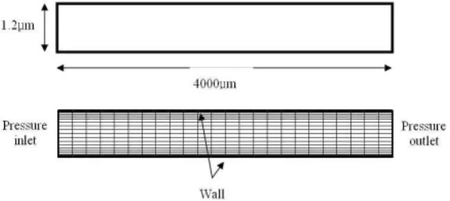
Fig. 1 Geometry and computational mesh of microchannel
2.2.MAXWELL SLIP CONDITION
A simple way to include the slip effect is to make a correction based on the degree of nonequilibrium near the wall surface that can be best represented by the shear stress. This idea can be traced to the work by Maxwell[5]
in which the following slip velocity boundary condition is proposed:
(6)
In this equation, , and represent the slip velocity, the shear stress on the wall and the slip coefficient, respectively. If we apply the linear theory to the constitutive equation of the shear stress and introduce the concept of diffusive reflection of the gas molecules near the surface as the collision in which a molecule is temporarily absorbed at the surface and then re-emitted, a slip model in the non-dimensional form can be written as
(7)
The is the Chapman-Enskog viscosity. The important parameter appearing in this model is the Knudsen number which measures the level of the slip induced by the gas-surface molecular interaction. The accommodation coefficient is usually chosen such that it fits to the experimental data and is tabulated for various gases and surfaces.
2.3.LANGMUIR SLIP CONDITION
An alternative way of describing slip can be developed by taking into account the interfacial interaction between the gas molecules and the surface molecules. It is well known from numerous studies of surfaces that gas molecules interact inelastically with the surface of the solid due to a long range attractive force: consequently, the gas molecules can get absorbed on the surface and then desorbed after some time lag. This is known in the literature as adsorption[2]. On the basis of this concept of adsorption, it is possible to develop a slip model for the gas-surface molecular interaction. If we model this interaction as a chemical reaction in which the gas molecule and the site form a complex, we may obtain an expression for the fraction of the surface covered by adsorbed atoms at thermal equilibrium, . With information about the fraction of the surface covered at
equilibrium determined by the Langmuir adsorption isotherm, the velocity slip can be expressed in term of , in the dimensional form[2],
(8)
Here subscript denotes a local value adjacent to the wall. For the simplest case, a monatomic gas at the stationary surface, the dimensionless slip velocity[3-4]
reduces to
(9)
where
and
exp
where is a function of molecular interaction parameter
, wall temperature , and the potential parameter of heat adsorption . The role of is very similar to the accommodation coefficient of the Maxwell model. For most molecular interaction models, the value of heat of adsorption falls under the range
kcal/mol. Its value may be inferred from experimental data or theoretical predictions of intermolecular forces.
2.4.NUMERICAL IMPLEMENTATION OF SLIP MODELS
In the context of the finite element method, the boundary conditions are treated by modifying the stiffness matrix. In order to explicitly demonstrate the implementation of slip models, the system of nonlinear equations equation (5) will be rewritten in the matrix form as follows:
(10)
where the subscript and represent the total number of variables and the node index at the solid wall, respectively. With the Langmuir slip model of a monatomic gas, the dimensionless slip velocity at the surface can be expressed, in Cartesian coordinates (), as follows
(11)
For the Maxwell slip model, the slip velocity is directly proportional to the normal gradient of the streamwise velocity component at the wall
(12)
In these slip models, is the reference pressure which is chosen as the pressure in the vicinity of the wall. As the equation (10) is solved iteratively, the slip velocity can be applied to the finite element matrix explicitly. At the iteration , the slip velocity is determined by using the Langmuir or Maxwell slip model in which the velocity and pressure are obtained from the previous step. The
equation (10) is then modified as
(13)
The new solutions are obtained by solving equation (13).
This process is repeated until the convergence is reached.
3. VERIFICATION AND VALIDATION
In order to validate the present numerical code, pressure-driven internal gas flows in a microchannel of high aspect ratio under isothermal condition are considered.
In addition to rarefaction effects associated with the microscale size, gas flows in a long microchannel with a significant pressure drop exhibit compressibility effects. For this reason, the flow is analyzed by considering the compressible equations, even though the characteristic speed may not be sufficiently high beyond the traditional threshold of Mach number 0.3.
In the present flow problem, the reference state is chosen as the exit conditions. The reference velocity is the area-averaged streamwise velocity at the channel exit. The geometry of the channel, computational mesh, and boundary conditions are depicted in Fig. 1. In the present work, a structured mesh with 525 points (25×21)
Fig. 2 Mass flow rate (kg/s) of helium gas in the scale of
depicted as a function of pressure ratio (Kn = 0.158)
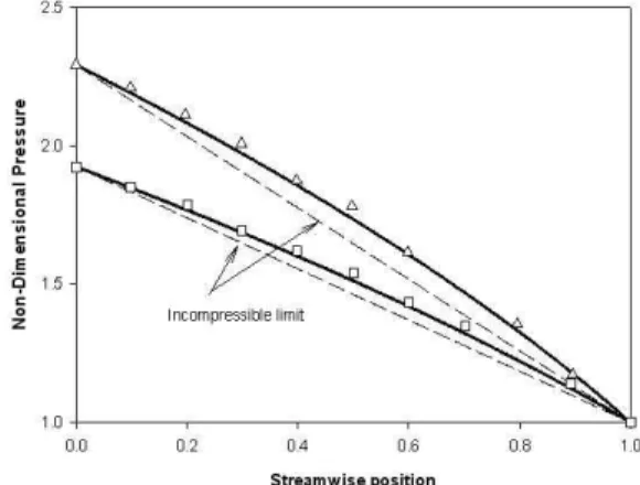
Fig. 3 Pressure distribution of helium gas along the micro- channel. Langmuir model by solid line; the experimental data by the symbols
Fig. 4 Mass flow rate (kg/s) of helium gas in the scale of
for different elements is used. The other important physical properties of helium
gas are
K atm Jkg⋅K
× N⋅sm
At the inlet and outlet of the channel, a pressure condition is prescribed. At the solid wall, the vertical velocity v vanishes and hence the streamwise velocity is equal to the slip velocity. The other variables at the boundary can be determined by solving the governing equations. In addition, the accommodation coefficient of the Maxwell model and the adsorption coefficient of the Langmuir slip model[3, p.112] are
or kcalmol
With the computational results in hand, comparisons with experimental and theoretical data[3,6] are performed for helium gas in Fig. 2-3. In Fig. 2, dimensional mass flow rates of helium gas in the microchannel are depicted as a function of the pressure ratio of inlet and outlet in a microchannel. Using the values assigned to the accommodation and adsorption coefficients, both slip models, Maxwell and Langmuir, seem to predict the experimental data correctly. It is also shown that the numerical results are in good agreement with the experimental and theoretical data even though the computational grid is quite coarse. Only a minor difference was found in the high pressure drop region owing to the higher order effects. The present analysis demonstrates that the same solution can be obtained if the accommodation coefficient of the Maxwell model and
the physical adsorption coefficient of Langmuir model are identical. This is a very surprising result since the two slip models were developed from totally different approaches. In Fig. 3, the pressure distribution along the channel is compared with that of the experimental data.
For comparison, the profile in the incompressibility limit is also given. The present numerical code seems to succeed in dealing with the nonlinearity of the pressure distribution and if the experimental uncertainties are considered, it can be said that the numerical solutions are in good agreement with the data. Furthermore, in order to check the accuracy of the present code, an analysis using linear and quadratic elements is conducted. Fig. 4 shows a comparison between the numerical and analytical data. A very coarse mesh with 50 points (5×10) is used to study the influence of order of the element. It is shown that there is a relatively big difference between the numerical and analytical results,
especially in the case of a high pressure difference when a linear element was utilized. However, the accuracy of the solution is greatly enhanced when a higher order of element, such as a quadratic element, is used. The tolerance between the numerical and analytical data reduces from 7.79% to 2.44% when a quadratic element is employed. It can be concluded that with a sufficient number of mesh points and a high order of element, the present numerical code can produce qualitatively correct results even in highly sensitive cases.
4. CONCLUSION
In this study, a numerical code based on the finite element method is developed for computational simulations of microscale fluid flow and heat transfer. Two slip models, Maxwell and Langmuir, are successfully implemented to describe the slip effect from gas-surface molecular interaction near the wall in internal flows of a long microchannel. Extension to the full Navier-Stokes-Fourier equations and generalized hydrodynamic models of highly nonequilibrium flow regimes will be the subject of future work.
ACKNOWLEDGEMENTS
This work was supported through Research Center for Aircraft Parts Technology by a grant from Korea Research Foundation (grant no. KRF-2008-005-J01002).
REFERENCES
[1] 2003, Reese, J.M., Gallis, M.A. and Lockerby, D.A.,
"New Direction in Fluid Dynamics: Non-equilibrium Aerodynamic and Microsystem Flows," Phil. Trans.
Roy. Soc. Lond. A, Vol.361, pp.2967-2988.
[2] 2002, Eu, B.C., Generalized Hydrodynamics: The Thermodynamics of Irreversible Processes and Generalized Hydrodynamics, Kluwer Academic Publisher.
[3] 2004, Myong, R.S., "Gaseous Slip Models Based on the Langmuir Adsorption Isotherm," Physics of Fluids, Vol.16, No.1, pp.104-117.
[4] 2006, Myong, R.S., "The Effect of Gaseous Slip on Microscale Heat Transfer: An Extended Graetz Problem," Int. J. Heat and Mass Transfer, Vol.49, pp.
2502-2513.
[5] 1879, Maxwell, J.C., "On Stresses in Rarefied Gases
Arising from Inequalities of Temperature," Phil. Trans.
Roy. Soc. Lond., Vol.170, pp.231-256.
[6] 1997, Arkilic, E.B., Schmidt, M.A. and Breuer, K.S.,
"Gaseous Slip Flow in Long Microchannels," Journal of Microelectromechanical System, Vol.6, No.2, pp.
167-178.
[7] 2004, Jang, J. and Wereley, S.T., "Pressure Distributions of Gaseous Slip Flow in Straight and Uniform Rectangular Microchannels," Microfluid Nanofluid, Vol.1, pp.41-51.
[8] 1999, Meinhart, C.D., Wereley, S.T. and Santiago, J.G., "PIV Measurements of a Microchannel Flow,"
Experiments in Fluids, Vol.27, pp.414-419.
[9] 1996, Beskok, A., Karniadakis, G.E. and Trimmer, W., "Rarefaction and Compressibility Effects in Gas Microflows," Transations of the ASME, Vol.118, pp.
448-456.
[10] 1997, Beskok, A. and Karniadakis, G.E., "Modeling Separation in Rarefied Gas Flows," AIAA Pap. No.
97-1883.
[11] 2008, Choi, H.I. and Lee, D., "Computations of Gas Microflows Using Pressure Correction Method with Langmuir Slip Model," Computers and Fluids, Vol.
37, No.10, pp.1309-1319.
[12] 2005, Choi, H.I., Lee, D.H. and Lee, D., "Complex Microscale Flow Simulations Using Langmuir Slip Condition," Numerical Heat Transfer; Part A:
Applications, Vol.48, No.5, pp.407-425.
[13] 2009, Kim, S.W., Kim, H.G. and Lee, D.,
"Numerical Analysis of the Slip Velocity and Temperature-Jump in Microchannel Using Langmuir Slip Boundary Condition," Transactions of the Korean Society of Mechanical Engineers, B, Vol.33, No.3, pp.
164-169.
[14] 2007, Kim, H.M. et al., "Langmuir Slip Model for Air Bearing Simulation Using the Lattice Boltzmann Method," IEEE Trans. Magnetics, Vol.43, No.6, pp.
2244-2246.
[15] 2009, Ahn, J.W. and Kim, C., "An Axisymmetric Computational Model of Generalized Hydrodynamic Theory for Rarefied Multi-Species Gas Flows,"
Journal of Computational Physics, Vol.228, No.11, pp.
4088-4117.
[16] 2009, Myong R.S. et al., "Fundamentals of Gas Flows in Thermal Nonequilibrium Learned from a Model Constitutive Relation," AIP Conference Proceedings, Vol.1084, pp.51-56.
[17] 2002, Chung, T.J., Computational Fluid Dynamics, Cambridge University Press.