A Branch and Bound Algorithm for Two-Stage Hybrid Flow Shop Scheduling : Minimizing the Number of Tardy Jobs
Hyun-Seon Choi․Dong-Ho Lee†*
Department of Industrial Engineering, Hanyang University, Seoul 133-791, Korea
2 단계 혼합흐름공정에서 납기 지연 작업수의 최소화를 위한 분지한계 알고리듬
최현선․이동호 한양대학교 산업공학과
This paper considers a two-stage hybrid flow shop scheduling problem for the objective of minimizing the number of tardy jobs. Each job is processed through the two production stages in series, each of which has multiple identical parallel machines. The problem is to determine the allocation and sequence of jobs at each stage. A branch and bound algorithm that gives the optimal solutions is suggested that incorporates the methods to obtain the lower and upper bounds. Dominance properties are also suggested to reduce the search space. To show the performance of the algorithm, computational experiments are done on randomly generated problems, and the results are reported.
Keywords: Two-stage hybrid flow shop, scheduling, number of tardy jobs, branch and bound
1. Introduction
A hybrid flow shop, alternatively called a flow shop with multiple processors, is an extended sys- tem of the ordinary flow shop. The hybrid flow shop consists of two or more production stages in series, but there exist one or more parallel ma- chines at each stage. The parallel machines are added to each stage of the flow shop for the ob- jective of increasing productivity and/or flexibility.
That is, it is natural to increase the system ca- pacity by adding machines at a certain production stage (Gupta, 1988). The flow of jobs is basically
unidirectional through the serial production stages, and each job can be processed by one of the par- allel machines at each stage. There may be finite buffers to decouple consecutive production stages.
Also, a certain amount of setup time may be re- quired when changing the product type at each machine.
This paper considers hybrid flow shop scheduling which is the problem of allocating jobs to parallel machines at each stage and sequencing the jobs al- located to each machine. Note that the two deci- sion variables are those of parallel machine sched- uling and flow shop scheduling. Hybrid flow shops are commonly found in the industries (Huang and
This work was supported by Korea Research Foundation Grant funded by Korean Government (MOEHRD) (KRF-2005-041-D00893). This is gratefully acknowledged.
†Corresponding author : Dong-Ho Lee, Department of Industrial Engineering, Hanyang University, Sungdong-gu, Seoul 133-791, Korea, Tel : +82-2-2220-0475, Fax: +82-2-2296-0471, E-mail : [email protected]
Received June 2006; revision received September 2006; accepted October 2006.
Li, 1998). For example, they can be found in the electronics industry such as printed circuit board manufacturing, semiconductor manufacturing, and lead frame manufacturing (Lee and Kim, 2004, Linn and Zhang, 1999). Also, a number of traditional industries, such as food, chemical and steel, have various types of hybrid flow shops (Tsubone et al., 1996).
The research articles on hybrid flow shop sched- uling can be classified using the performance mea- sures used, i.e., those without due-date such as makespan and total flow time and those with due- date such as maximum tardiness, number of tardy jobs and mean tardiness. (See Linn and Zhang, 1999 for a literature review.) Gupta and Tunc (1991) con- sider the problem with the objective of minimizing makespan and suggest heuristic algorithms. Other heuristics for minimizing makespan are suggested by Lee and Vairaktarakis (1994), Chen (1995) and Lee and Park (1999) that consider two-stage hybrid flow shop. Fouad et al. (1998) consider a three- stage hybrid flow shop scheduling problem occur- red in the woodworking industry and suggest heu- ristic algorithms. Brah and Hunsucker (1991) sug- gest branch and bound algorithms that minimize makespan, and later, their lower bounds were im- proved by Moursli and Pochet (2000). Also, Azizoglu et al. (2001) consider the problem with the objec- tive of minimizing total flow time and suggest a branch and bound algorithm.
Several research articles consider due-date based measures. Guinet and Solomon (1996) suggest the list scheduling algorithms for multi-stage hybrid flow shop scheduling with the objective of minimizing maximum tardiness. Here, the list scheduling algo- rithms list the jobs in some order using a priority rule and assigns them to the machines according to this order. Gupta and Tunc (1998) consider the two- stage hybrid flow shop scheduling with the ob- jective of minimizing the number of tardy jobs and suggest several heuristic algorithms. Here, a tardy job is defined as the job whose completion time is greater than its due date. Recently, Lee and Kim (2004) considered a two-stage hybrid flow shop with parallel machines only at the first stage and suggested a branch and bound algorithm that mini- mizes total tardiness. Later, Lee et al. (2004) ex- tended their research to multi-stage hybrid flow shop and suggested a bottleneck-focused heuristic for the
objective of minimizing total tardiness. In this heu- ristic, a schedule for the bottleneck stage is first constructed and then the schedules for the other stages are constructed based on that for the bott- leneck.
This paper focuses on a scheduling problem in two-stage hybrid flow shops with the objective of minimizing the number of tardy jobs. The objective considered in this paper is important in many cases since the cost penalty incurred by a tardy job does not depend on how late it is, but the fact that it is late. For example, a late job may cause a customer to switch to another supplier, especially in the just- in-time production environment (Ho and Chang, 1995).
As noted in the previous research articles, the pro- blem considered in this paper is an NP-hard pro- blem. This can be easily seen from the fact that the parallel machine scheduling problem that mini- mizes the number of tardy jobs is NP-hard (Garey and Johnson, 1979). As stated earlier, the objective of minimizing the number of tardy jobs is dealt with by Gupta and Tunc (1998) that considers a two-stage hybrid flow shop with only one machine at the first stage. Unlike this, we focus on general two-stage hybrid flow shops in which two or more machines exist at each stage. In addition, we sug- gest a branch and bound algorithm that gives opti- mal solutions. The methods to obtain the lower and upper bounds are suggested and also dominance properties are derived to reduce the solution space.
To show the performance of the algorithm, compu- tational experiments are performed on randomly generated problems, and the results are reported.
This paper is organized as follows. In the next section, the problem considered here is described in more detail with a mathematical formulation. The branch and bound algorithm is presented in Section 3, and the results of computational test are repor- ted in Section 4. Finally, Section 5 concludes the paper with a short summary and discussions on po- ssible extensions.
2. Problem Description
Before describing the problem considered in this paper, we present the structure of the two-stage hybrid flow shop. As stated earlier, the two-stage
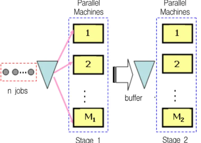
hybrid flow shop consists of two serial stages, al- ternatively called workstations in the literature, but there exist one or more identical parallel machines at each stage. In Figure 1, Mk denotes the number of machines at stage k, k = 1, 2. Each job consists of two operations, i.e., the first (second) one is processed on one of the parallel machines at the first (second) stage. Here, the operations are proc- essed sequentially, without overlapping between stages.
Figure 1. Two-stage hybrid flow shop : a schematic view
As stated earlier, there are two types of decision variables in the two-stage hybrid flow shop sched- uling problem considered in this paper. They are;
(a) allocating jobs to the parallel machines at each stage and (b) sequencing the jobs allocated to each machine. The objective is to minimize the number of tardy jobs, i.e.,
minimize
,
where Ti = max{0, Ci - di} and (a) = 1 if a > 0, and 0 otherwise. Here, Ci and di denote the com- pletion time and the due date of job i, respectively.
Note that the completion times of jobs depend on the two decision variables, allocation and sequenc- ing, and the problem considered here is to de- termine them for the objective of minimizing the number of tardy jobs in the general two-stage hy- brid flow shop.
This paper considers a static and deterministic scheduling problem. That is, all jobs are ready for processing at time zero, i.e., zero ready time, and job descriptors such as processing times and due dates are deterministic and given in advance. It is
assumed that the parallel machines at each stage are identical and hence processing time of an oper- ation at each stage is the same for each of the ma- chines at that stage. Other assumptions made in the problem considered here are : (a) no job can be split or pre-emptied; (b) each machine can process only one job at a time and each job can be processed on one machine; (c) machine breakdowns are not considered; and (d) the buffer capacity between the two stages is infinite.
The hybrid flow shop scheduling problem consid- ered in this paper can be formulated as an integer programming model. First, the notations used are summarized below.
Parameters
Mk number of identical machines at stage k, k
= 1, 2
di due date of job i, i = 1,…, N pik processing time of job i at stage k V large number
Decision variables
xijmk = 1 if job j is processed directly after job i on machine m at stage k, and 0 other- wise (x0jmk = 1 if job j is the first job to be processed on machine m at stage k and xi0mk= 1 if job i is the last job to be proc- essed on machine m in stage k.)
cik completion time of job i at stage k
Now, the integer programming model, modified from that of Guinet and Solomon (1996), is given as follows.
Minimize
subject to
= 1 for all j, k and i ≠ j (1)
= 1 for all m and k (2)
≠
≠
= 0 for all h, m and k (3)
≥
⋅ for all j, k andParallel Machines
Parallel Machines
Stage 2 Stage 1
buffer n jobs
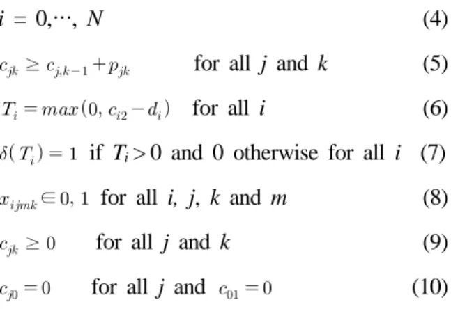
i = 0,…, N (4)
≥ for all j and k (5)
for all i (6)
if Ti> 0 and 0 otherwise for all i (7)
∈ for all i, j, k and m (8)
≥ for all j and k (9)
for all j and (10) The objective function denotes minimizing the number of tardy jobs, where the tardiness of each job is specified in constraint (6). Constraint (1) en- sures that each job is processed once and once on- ly at each stage. Constraint (2) specifies that each machine must be assigned to one job at most.
Note that x0jmk= 1 if job j is the first job to be pro- cessed on machine m at stage k. Similarly, xi0mk= 1 if job i is the last job to be processed on machine m in stage k. Constraints (3) ensure that each job has a predecessor and a successor on its machine.
The job completion time at each machine is repre- sented by constraints (4) and (5). In other words, constraint (4) implies that if job j is processed di- rectly after job i on machine m at stage k, the com- pletion time of job j at stage k is larger than or equal to the sum of the completion time of job i at stage k and the processing time of job j at stage k. Also, constraint (5) implies that the completion time of job j at stage k is larger than or equal to the sum of the completion time of job j at stage k - 1 and the processing time of job j at stage k. Con- straints (7) specify the number of tardy jobs. Final- ly, the other constraints (8), (9) and constraints (10) are the conditions on the decision variables.
3. Branch and Bound Algorithm
This section presents the branch and bound (B&B) algorithm suggested in this paper. First, we present the branching scheme that generates all possible schedules. Then, the methods to obtain the lower and upper bounds are suggested. As in the ordinary B&B algorithm, each node of the B&B tree can be deleted from further consideration (fathomed) if the lower bound at the node is great-
er than or equal to the incumbent solution value, i.e., the smallest upper bound of all nodes obtained so far. Finally, the dominance properties are sug- gested to reduce the search space.
3.1 Branching
To generate all possible solutions, we adopt the idea of Azizoglu et al. (2001) that consider the problem with minimizing total flow time. The en- tire B&B tree consists of two subtrees in series, each of which represents N! orderings of jobs at each stage of the hybrid flow shop. In the first subtree, N nodes are branched from the root node (level 1), N - 1 nodes from each node at the second level, and so on. Also, the second subtree starts from each of the leaf nodes of the first subtree.
That is, N nodes are branched at level N + 1, N - 1 nodes at the level N + 2, and so on. In this way, we can generate (N!)2 orderings of jobs.
Each node of the first (second) subtree corre- sponds to a partial schedule at the first (second) stage. More specifically, at each node, a set of jobs can be specified by going back on the path from that node toward the root node, and each of these jobs are allocated and sequenced to the earlier av- ailable machine in sequence. In this way, we can generate all possible allocation and sequence at each stage of the hybrid flow shop since we con- sider the regular measure of performance. See Azizoglu et al. (2001) for more details on how the
1 2 3
2 3
3 2
2
1 3
3
3 2
2
subtree
for the second stage level 1
level 2
level 3 subtree
for the first stage
root node
Figure 2. Branch and bound tree: example
B&B tree explained here can generate all feasible schedules. <Figure 2> shows an example of the B&B tree for a problem with 3 jobs. It can be seen from the figure that this method determines the job schedule from the first to the second stage.
For node selection (or branching), the depth-first rule is used in this study. In this rule, if the cur- rent node is not fathomed, the next node to be considered is one of its child node, i.e., the node with the smallest index.
3.2 Bounding
3.2.1 Obtaining the lower bound
The lower bound suggested in this paper is com- puted at each node of the B&B tree. As stated earlier, each node of the B&B tree corresponds to a partial schedule and the lower bound is computed by estimating the smallest (and also infeasible) com- pletion time of each job at the second stage. To do this, we use the partial schedule and the jobs not included in the partial schedule. Let PSl denote the set of jobs included in the partial schedule at node l.
Two cases are considered in the computation of the lower bound.
Case 1 : When the current node l is at the first subtree
In this case, the lower bound at node l is calcu- lated by
NT1 + NT2,
where NT1 is the number of tardy jobs calculated for those in the partial schedule PSl and NT2 is the number of tardy jobs derived from those not in PSl.
First, NT1 is calculated by estimating the smallest (but infeasible) completion time of each job in PSl
at the second stage. That is, the smallest com- pletion time of each job can be set as
where φT is the ready time of the earliest available machine at the second stage and cik, as defined earlier, is the completion time of job i at stage k.
Here, the earliest available machine at the second stage implies the one with the smallest completion
time of the last scheduled job among those in PSl. Note that the smallest completion time of a job given above is always smaller than the completion time of that job in the optimal schedule. This is because the delay times are ignored when calculat- ing NT1. Then, the number of tardy jobs NT1 can be calculated by comparing the smallest completion time and due date of each job in PSl. That is,
∈
, where Ti = max{0, ci2- di} for i∈PSl.
Second, NT2 is calculated by aggregating the two-stage hybrid flow shop scheduling problem in- to the single machine problem that minimizes the number of tardy jobs. In this method, the process- ing time of job i∉ PSl at the second stage is modified as
′ ,
i.e., job splitting is allowed, and the corresponding single machine scheduling problem is solved using the optimal algorithm of Moore (1968). Then, NT2
is set to the number of tardy jobs obtained from the single machine problem. That is,
∉
,
where Ti = max{0, ci - di} for i∉ PSl. Note that ci is the completion time of job i obtained by the algorithm of Moore (1968). Note that NT2 is a val- id lower bound for the jobs not in PSl since it is assumed that each unscheduled job is completed at the first stage before its release time at the second stage. Also, the single machine scheduling problem is solved using the modified processing time, i.e., processing time divided by the number of parallel machines at the second stage.
Case 2 : When the current node l is at the second subtree
Like the method of case 1, the lower bound in this case is calculated by
NT1 + NT2.
Here, NT1 is calculated using the method of the first case, i.e., estimating the smallest (but in- feasible) completion time of each job at the second
stage. More formally,
∈
,
where Ti = max{0, ci2- di} for i∈PSl. Here, ci2 is the completion time of job i at the second stage and can be obtained directly from the partial sche- dule. On the other hand, NT2 for i ∉ PSl is calcu- lated by estimating the completion time as
.
Note that in this case, the waiting time of un- scheduled jobs at the second stage, i.e., max{0, ci1
-φT}, is ignored. Therefore, NT2 is a valid lower bound for the jobs not in PSl.
3.2.2 Obtaining the upper bound
The initial upper bound, i.e., an initial feasible solution value, at the root node of the B&B tree is obtained using the list scheduling approach. As stated earlier, the list scheduling method lists the jobs in some order using a priority rule and as- signs them to the machines according to this order.
In this paper, we use two priority rules, EDD (ear- liest due date) and MST (minimum slack time).
The EDD rule is used after modifying the due date of each job as
′ .
Then, the jobs are ordered in the non-decreasing order of ′, and they are allocated to machines ac- cording to this order. Note that each job is allo- cated to the earliest available machine as in the bran- ching scheme explained earlier. Also, the MST rule is the same as the EDD rule except that the jobs are ordered according to the non-decreasing order of slack time. Here, the slack time is defined as
.
Now, the intial upper bound is set to the mini- mum of those obtained by the two rules and up- dated whenever a better (feasible) solution is ob- tained at each leaf node of the B&B tree.
3.3 Dominance properties
To reduce the search space of our B&B algo- rithm, two properties are derived in this paper. The first property, which is given blow and its proof is
omitted here since it is given in Azizoglu and Kirca (1998), specifies the condition that a job should be positioned last at the first stage of the hybrid flow shop. That is, a job satisfying the condition of proposition 1 is never tardy in any positions and hence can be sequenced last.
Proposition 1. There exists an optimal schedule in which job w is processed at the last position on any one of the machines at the first stage if
′ ≥
,
where ′= - .
The second property specifies the condition that partial schedule σyi is dominated by σyj, where σyi is the partial schedule obtained by appending job i (not in σ) to the end of partial schedule σ. From this property, we can see that job i should be posi- tioned last at the first stage of the hybrid flow shop.
Proposition 2. For any partial schedule σ at the first stage, σyi is dominated by σyj if
pi1 > pj1 and φT + pi1 + pi2 > di,
where i and j denote indices for the (unscheduled) jobs not in partial schedule σ and φT is the ready time of the earliest available machine correspond- ing to the partial schedule σ.
Proof. Let c(σyj)1 denote the completion time of job j of partial schedule σyj at the first stage. Two cases can be considered.
Case 1 : c(σyj)1 + pj2 > dj
In this case, jobs i and j are both tardy jobs at the first stage since φT+ pi1+ pi2 >
di and c(σyj)1 + pj2 > dj. Hence, the num- ber of tardy jobs of partial schedule σyi is the same as that of σyj.
Case 2 : c(σyj)1 + pj2 ≦ dj
In this case, job j may not be a tardy job and hence it is better to position job i to the last position since pi1> pj1. In other words, the unscheduled jobs can be moved earlier, which results that the number of tardy jobs of partial schedule σyj is less than or equal to that of σyi.
Therefore, the number of tardy jobs for partial schedule σyj is less than that of σyi. This com- pletes the proof.
4. Computational Experiments
To show the performance of the B&B algorithm suggested in this paper, computational tests were done on randomly generated test problems, and the results are reported in this section. The algorithm was tested with respect to two performance measures.
They are the number of problems that the B&B al- gorithm gave the optimal solutions within 5000 seconds and CPU seconds. Here, the time limit was set because the B&B algorithm may not give the optimal solutions for large-sized test problems. The algorithm was coded in C++ and the test was per- formed on a workstation with an Intel Xeon pro- cessor operating at 3.20 GHz clock speed.
For the test, 960 problems were generated ran- domly, i.e., 10 problems for each of 96 combina- tions of the number of machines (1, 2, 3 and 4 at the first stage and 2, 3 and 4 at the second stage), four levels of the number of jobs (10, 12, 14 and 15), and two levels of the due date tightness (loose, tight). The processing times were generated from DU(10, 40), where DU(a, b) is the discrete uni- form distribution with range [a, b]. Due dates were generated using the method of Gupta (1998). That is, they were generated from DU(p, p), where α and ( >) were set to 0.6 (0.2) and 0.8 (0.4) for the case of loose (tight) due dates and p was set as
.
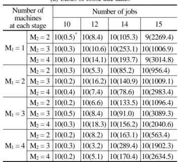
Test results are summarized in <Table 1> that shows the number of problems that the B&B algo- rithm gave the optimal solutions within 5000 sec- onds and average CPU seconds (in parenthesis). It can be seen from the table that the B&B algorithm gives the optimal solutions for most test problems.
In fact, the B&B algorithm gave the optimal sol- utions up to the problems with 14 jobs for loose due dates and 12 jobs for tight due dates. Also, we can see that the number of machines at each
stage plays an important role in the problem complexity. That is, the test problems having rela- tively large number of machines at the first stage were easier to solve since Proposition 2 considers the parallel machines at the first stage. Also, the computation times for the problems with loose due dates are smaller than those for the problems with tight due dates. However, the computation times of both cases increase significantly when the number of jobs increases due to the inherent complexity of the problem.
Table 1. Performance of the algorithm (a) Cases of loose due dates Number of
machines at each stage
Number of jobs
10 12 14 15
M1= 1
M2= 2 10(0.5)* 10(8.4) 10(105.3) 9(2269.4) M2= 3 10(0.3) 10(10.6) 10(253.1) 10(1006.9) M2= 4 10(0.4) 10(14.1) 10(193.7) 9(3014.8)
M1= 2
M2= 2 10(0.3) 10(5.3) 10(85.2) 10(956.4) M2= 3 10(0.2) 10(16.2) 10(140.9) 10(1009.1) M2= 4 10(0.4) 10(7.4) 10(78.6) 10(2983.4)
M1= 3
M2= 2 10(0.2) 10(6.6) 10(133.5) 10(1096.4) M2= 3 10(0.5) 10(8.4) 10(91.0) 10(3089.3) M2= 4 10(0.3) 10(18.3) 10(156.2) 10(2040.6)
M1= 4
M2= 2 10(0.2) 10(8.2) 10(163.1) 10(563.4) M2= 3 10(0.3) 10(3.2) 10(289.4) 10(1902.3) M2= 4 10(0.2) 10(5.1) 10(170.4) 10(2634.5)
* number of problems that the B&B algorithm gave the optimal solutions out of 10 problems and CPU seconds (in parenthesis)
(b) Cases of tight due dates Number of
machines at each stage
Number of jobs
10 12 14 15
M1= 1
M2= 2 10(2.8) 10(12.3) 10(585.3) 8(2625.3) M2= 3 10(1.2) 10(10.6) 10(725.3) 8(3025.1) M2= 4 10(1.1) 10(15.7) 9(663.4) 7(1005.6)
M1= 2
M2= 2 10(0.5) 10(6.3) 10(383.3) 9(2006.4) M2= 3 10(0.9) 10(15.8) 10(425.6) 10(3523.2) M2= 4 10(0.7) 10(13.8) 10(528.9) 9(4019.3)
M1= 3
M2= 2 10(0.6) 10(9.5) 10(631.5) 10(1263.4) M2= 3 10(2.0) 10(3.1) 10(226.4) 10(1991.6) M2= 4 10(1.5) 10(15.3) 10(341.6) 9(2536.1)
M1= 4
M2= 2 10(0.9) 10(6.9) 10(163.8) 10(1094.2) M2= 3 10(1.6) 10(17.5) 10(512.3) 10(1697.2) M2= 4 10(1.3) 10(8.6) 10(226.7) 10(2463.8) See the footnotes of (a).
5. Concluding Remarks
The paper considered a two-stage hybrid flow shop scheduling problem for the objective of minimizing the number of tardy jobs. Unlike the previous re- search, we focused on general two-stage hybrid flow shops in which two or more machines exist at both stages and suggested a branch and bound algorithm that gives optimal solutions. The methods to calculate lower and upper bounds are suggested, and two properties that characterize the optimal solutions were also derived to reduce the search space. Test results of computational experiments showed that the B&B algorithm suggested in this paper gave the optimal solutions for moderate-sized test problems within a reasonable amount of com- putation time.
This research can be extended in several direc- tions. First, it is needed to develop more efficient algorithms to solve practical-sized problems. To do this, it may be necessary to develop heuristic algo- rithms rather than the optimal algorithm. Second, it is worth to consider the problem in which the buf- fer size between the two stages is finite. Also, to make the research more practical, the problem should be extended to the systems with more than two stages. In this case, the simulation study, together with dispatching rules, may be more applicable.
Finally, the hybrid flow shops with uniform or un- related parallel machines at each stage can be a practical extension.
References
Azizoglu, M., Cakmak, E., and Kondakci, S. (2001), A flexible flow shop problem with total flow time minimization, European Journal of Operational Research, 132, 528-538.
Azizoglu, M. and Kirca, O. (1998), Tardiness mini- mization on parallel machines, International Journal of Production Economics, 55, 163-168.
Brah, S. A. and Hunsucker, J. L. (1991), Branch and bound algorithm for the flow shop with multiple processors, European Journal of Operational Research, 51, 88-99.
Chen, B. (1995), Analysis of classes of heuristics for scheduling a two-stage flow shop with paral- lel machines at on stage, Journal of the Opera- tional Research Society, 46, 231-244.
Fouad, R., Abdelhakim, A. and Salah, E. E. (1998),
A hybrid three-stage flowshop problem Efficient heuristics to minimize makespan, European Journal of Operational Research, 109, 321-329.
Garey, M. R. and Johnson, D. S. (1979), Computers and Intractability : A Guide to the Theory of NP- Completeness, W. H. Freeman and Company.
Guinet, A. G. P. and Solomon, M. M. (1996), Scheduling hybrid flowshops to minimize max- imum tardiness or maximum completion time, International Journal of Production Research, 34, 1643-1654.
Gupta, J. N. D. (1988), Two-stage hybrid flow shop scheduling problem, Journal of the Opera- tional Research Society, 39, 359-364.
Gupta, J. N. D. and Tunc, E. A. (1991), Schedu- ling for a two-stage hybrid flowshop with paral- lel machines at the second stage, International Journal of Production Research, 29, 1480-1502.
Gupta, J. N. D. and Tunc, E. A. (1998), Minimi- zing tardy jobs in a two-stage hybrid flowshop, International Journal of Production Research, 36, 2397-2417.
Ho, J. C. and Chang, Y-L. (1995), Minimizing the number of tardy jobs for m parallel machines, European Journal of Operational Research, 84, 343-355.
Huang, W. and Li, W. (1998), A two-stage hybrid flowshop with uniform machines and setup times, Mathematical and Computer Modelling, 27, 27-45.
Lee, C. Y. and Vairaktarakis, G. L. (1994), Minimi- zing makespan in hybrid flow shops, Operations Research Letters, 16, 149-158.
Lee, G.-C. and Kim, Y.-D. (2004), A branch-and- bound algorithm for a two-stage hybrid flow shop scheduling problem minimizing total tardiness, International Journal of Production Research, 42, 4731-4743.
Lee, G.-C., Kim, Y.-D. and Choi, S.-W. (2004), Bottleneck-focused scheduling for a hybrid flow shop, International Journal of Production Research, 42, 165-181.
Lee, J.-S. and Park, S.-H. (1999), Scheduling heu- ristics for a two-stage hybrid flowshop with non- identical parallel machines, Journal of the Korean Institute of Industrial Engineers, 25, 254-265.
Linn, R. and Zhang, W. (1999), Hybrid flow shop scheduling, Computers and Industrial Engineering, 37, 57-61.
Moore, J. M. (1968), An n-job, one-machine se- quencing algorithm for minimizing the number of jobs, Management Science, 15, 102-109.
Mourisli, O. and Pochet, Y. (2000), A branch-and- bound algorithm for the hybrid flow shop, Inte- rnational Journal of Production Economics, 64, 113-125.
Tsubone, H., Ohba, M. and Uetake, T. (1996), The impact of lot sizing and sequencing on manu- facturing performance in a two-stage hybrid flow shop, International Journal of Production Research, 34, 3037-3053.