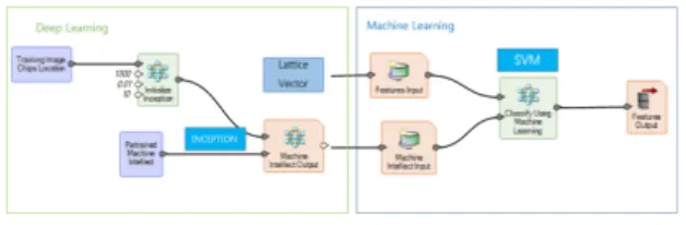
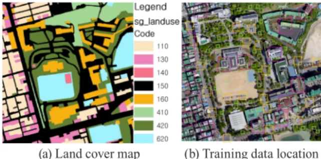
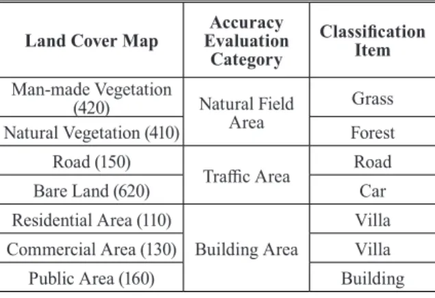
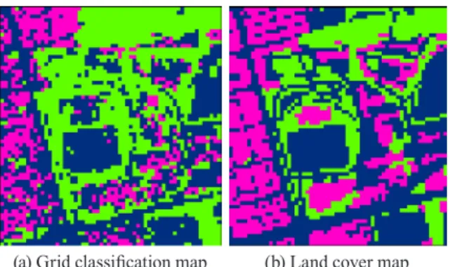
Automatic Classification of Drone Images Using Deep Learning and SVM with Multiple Grid Sizes
8
0
0
전체 글
(2)
(3)
(4)
(5)
(7)
(8)
수치
+2
관련 문서
● Define layers in Python with numpy (CPU only).. Fei-Fei Li & Justin Johnson & Serena Yeung Lecture 8 - 150 April 27,
: Model Parallelism in Deep Learning is NOT What You Think : Paper, Efficient and Robust Parallel DNN Training through Model Parallelism on Multi-GPU Platfrom,
If local computing power is selected, the drone platform runs the standard q-learning prediction algorithm and updates the Q-table, then reads the sensor's SINR data,
Preliminary Study of IR Sensor Equipped Drone-based Nuclear Power Plant Diagnosis Method using Deep Learning. Ik Jae Jin and
Motivation – Learning noisy labeled data with deep neural network.
High school Japanese I textbooks were analyzed based on the classification of culture types based on Finocchiaro & Bonomo, Chastain's theory and
If we wish to develop a learning process based on
This study aims to analyze the process and the features of corporate e-Learning as a form of informal learning. For this purpose, the concept of
