On the ratio of two independent weighted Lindley variables^†

On the ratio of two independent weighted Lindley variables ^†

Changsoo Lee ¹ · Kyungsu Ahn ²

12 Department of Flight Operation, Kyungwoon University

Received 12 December 2018, revised 2 May 2019, accepted 4 May 2019

Abstract

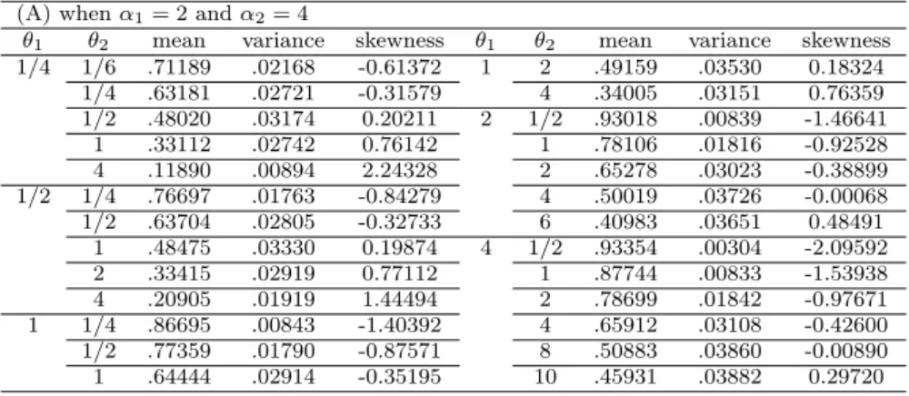
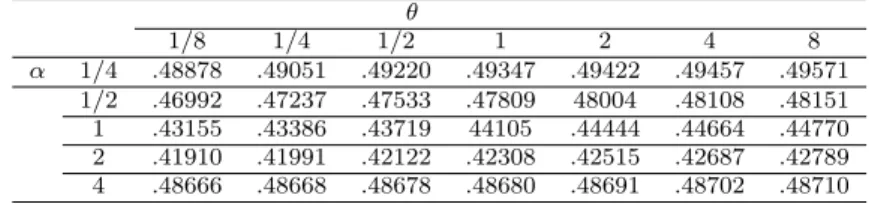
We shall consider the distribution for the ratio based on two independent two pa- rameter Lindley random variables and two independent weighted Lindley random vari- ables respectively. We shall observe the skewness for each the ratio and shall study numerically trends for the skewness for each the ratio based on two independent two parameter Lindley random variables and two independent weighted Lindley random variables. We shall consider the correlation coefficient between two variables having a bivariate weighted Lindley density based on the weighted Lindley density.

Keywords: Bivariate weighted Lindley density, correlation coefficient, IFR, Lindley dis- tribution, weighted Lindley density.

1. Introduction

Many authors have studied estimations for the reliability and parameters in the Lindley distribution. Ghitany et al. (2008) studied applications for the Lindley distribution. Krishna and Kumar (2011) and Khamnei (2013) considered reliability estimations for one parameter Lindley distribution with progressively type II right censored sample and an outlier respec- tively. Elbatal et al. (2013) considered the MLE in a generalized Lindely distribution based on a mixture of two gamma density. Damsesy et al. (2015) considered the reliability and the failure rate of the electronic by using mixture Lindley distribution, which its distribution has been applied to the life times of the electronic unit in the system.

Investment managers, traders and analysts find it very important to calculate correlation, because the risk reduction benefits of diversification rely on this statistic. Financial spread- sheets and software can calculate the value of correlation quickly. For example, it can be helpful in determining how well a mutual fund performs relative to its benchmark index, or another fund or asset class. By adding a low or negatively correlated mutual fund to an existing portfolio, the investor gains diversification benefits. And the skewness is very important in portfolio management, risk management, option pricing, and trading.

† This research is supported by 2019 Kyungwoon University Research Fund.

1

Corresponding author: Associate professor, Department of Flight Operation, Kyungwoon University, Gumi 730-850, Korea. E-mail: [email protected]

2

Assistant professor, Department of Flight Operation, Kyungwoon University, Gumi 730-850, Korea.

In this paper, we consider the distribution for the ratio based on two independent two parameter Lindley random variables and two independent weighted Lindley random variables respectively, and we observe the skewness for each the ratio and shall study numerically trends for the skewness for each the ratio based on two independent two parameter Lindley random variables and two independent weighted Lindley random variables respectively. And we shall consider the correlation coefficient between two variables having a bivariate weighted Lindley density based on the weighted Lindley density.

2. Two-parameter Lindley distribution

2.1. Failure rate of two parameter Lindley distribution

A two parameter Lindley density is as given in Shanker et al. (2013) :

f (x) = θ ²

θ + β (1 + βx)e ^−θx , x > 0, (2.1) where θ(> 0) is the shape parameter and β(> 0) is the scale parameter.

It is a mixture of an exponential distribution and a gamma distribution, and a special density of a generalized Lindley distribution based on a mixture of two gamma distributions in Elbatal et al. (2013), and also it is one parameter Lindley density when β = 1.

Let X be a random variable having the density function (2.1). Then its cumulative distri- bution function (cdf) is given:

F (x) = 1 − e ^−θx − θβ

θ + β xe ^−θx , for 0 < x. (2.2) From the definition and a property of an increasing failure rate (IFR) in Saunders (2007), we can obtain the following:

Proposition 2.1 Let X be a life time variable having the density function (2.1). Then, the distribution F (x) having (2.2) is an IFR.

Proof Let f (x) be the density having (2.1). Then _dx ^d

log f (x) = − _(1+βx) ^β

< 0 for 0 < x, and then log f (x) is a concave function on (0, ∞). Thus the density function f (x) is the Polya frequency function of order two and then from Theorem 11 of Section 4.7 in Saunders (2007), the Lindley distribution F (x) is IFR.

2.2. Distribution of the ratio

Assume X and Y be independent two parameter Lindley random variables with the density function (2.1) each having parameters (β 1 , θ 1 ) and (β 2 , θ 2 ) respectively.

Then from the quotient density function of two independent random variables in Rohatgi

(1976) and formula 3.381 (4) in Gradshteyn and Ryzhik (1965), the density function for

W = X/Y is given :

f W (w) = θ ² ₁ θ ₂ ² (θ 1 + β 1 )(θ 2 + β 2 )

"

1

(θ 1 w + θ 2 ) ² + 2(β 1 w + β 2 ) (θ 1 w + θ 2 ) ³ + 6β 1 β 2 w

(θ 1 w + θ 2 ) ⁴

#

, for w > 0. (2.3)

Let R = Y /(X + Y ) be the ratio for two independent two parameter Lindley random variables with the density function (2.1) each having parameters (α 1 , θ 1 ) and (α 2 , θ 2 ), re- spectively.

Then R = 1/(1 + W ) and dw = −dr/r ² , and then from the density function (2.3) of W , the density function of the ratio R is given:

f _R (r) = θ ² ₁ θ ² ₂ (θ ₁ + β ₁ )(θ ₂ + β ₂ )

"

1

(θ ₁ (1 − r) + θ ₂ r) ² + 2(β 1 (1 − r) + β 2 r) (θ ₁ (1 − r) + θ ₂ r) ³ + 6β 1 β 2 r(1 − r)

(θ ₁ (1 − r) + θ ₂ r) ⁴

#

, for 0 < r < 1. (2.4)

From the density function (2.4) for the ratio R, k-th moments for the ratio R can’t be represented by a closed form, but it can be computed numerically by uniform convergence of k-th moments of the ratio R over [0, 1], we can obtain numerical values of approximate means, variances, and coefficients of the skewness for0 the ratio density function when values for parameters (β 1 , θ 1 ) and (β 2 , θ 2 ) are as given in Table 2.1.

From Table 2.1, we can observe the following fact:

Fact 2.2 Assume X and Y be independent two-parameter Lindley random variables with the density function (2.1) each having parameters (β 1 , θ 1 ) and (β 2 , θ 2 ) respectively. Then

(A) when scale parameters β 1 = β 2 = 1,

(i) the coefficient of the skewness of the density function (2.4) of the ratio R is zero only when θ 1 = θ 2 .

(ii) the density function (2.4) is right skewed when θ ₂ > θ ₁ , it is left skewed when θ ₂ < θ ₁ .

(B) when the scale parameters β ₁ = 1 < β ₂ = 2, the density function (2.4) is right skewed when θ ₂ > θ ₁ , but it’s left skewed when θ ₂ ≤ θ ₁ .

(C) when the scale parameters β 1 = 2 < β 2 = 1, the density function (2.4) is right skewed

when θ 2 ≥ θ 1 , but it is left skewed when θ 2 < θ 1 .

Table 2.1 Approximate means, variances, coefficients of skewness for the ratio (A) when β

= β

= 1

θ

θ

mean variance skewness θ

θ

mean variance skewness 1/4 1/6 0.58567 0.05792 -0.34492 1 2 0.35618 0.06942 0.62549

1/4 0.50000 0.06200 0.00000 4 0.23771 0.05279 1.29945 1/2 0.35347 0.05766 0.61894 2 1/4 0.86597 0.02556 -2.28792 1 0.22663 0.04238 1.34606 1/2 0.77141 0.04734 -1.35585 2 0.13403 0.02556 2.28794 1 0.64382 0.06942 -0.62549 4 0.07544 0.01355 3.58792 2 0.50000 0.07963 0.00000 1/2 1/4 0.64653 0.05766 -0.61894 4 0.36365 0.07358 0.59176 1/2 0.50000 0.06952 0.00000 4 1/4 0.92456 0.01355 -3.58776 1 0.35254 0.06370 0.63570 1/2 .86034 0.02981 -2.23789 2 0.22859 0.04734 1.35586 1 .76229 0.05279 -1.29946 4 0.13968 0.02981 2.23791 2 .63635 0.07358 -0.59176 1 1/4 0.77337 0.04238 -1.34606 4 .50000 0.08200 0.00000 1/2 0.64746 0.06370 -0.63570 6 .42304 0.07998 0.32447

1 0.50000 0.07500 0.00000 8 .37169 0.07597 0.55383

(B) when β

= 1 < β

= 2

θ

θ

mean variance skewness θ

θ

mean variance skewness 1/4 1/6 0.59718 0.05504 -0.36084 1 2 0.38084 0.06994 0.52230

1/4 0.51481 0.05941 -0.29110 4 0.25384 0.05498 1.19860 1/2 0.37233 0.05694 0.55983 2 1/4 0.87700 0.02109 -2.37084 1 0.24471 0.04380 1.24539 1/2 0.79145 0.04032 -1.46838 2 0.14692 0.02748 2.13756 1 0.67152 0.06277 -0.74210 4 0.08205 0.01475 3.39368 2 0.52778 0.07701 -0.10632 1/2 1/4 0.66195 0.05319 -0.65132 4 0.38387 0.07453 0.50287 1/2 0.52222 0.06506 -0.06117 4 1/4 0.93249 0.01042 -3.77723 1 0.37659 0.06348 0.54522 1/2 0.87611 0.02379 -2.43226 2 0.24749 0.04942 1.23941 1 0.78652 0.04515 -1.46384 4 0.15058 0.03180 2.10609 2 0.66355 0.06812 -0.71715 1 1/4 0.78728 0.03721 -1.39107 4 0.52222 0.08062 -0.08965 1/2 0.67010 0.05756 -0.71123 6 0.44033 0.08025 0.25225 1 0.52778 0.07145 -0.09472 8 0.38542 0.07687 0.49225

(C) when β

= 2 > β

= 1

θ

θ

mean variance skewness θ

θ

mean variance skewness 1/4 1/6 0.57210 0.05649 -0.31552 1 2 0.32848 0.06277 0.74212

1/4 0.48519 0.05941 0.02911 4 0.21348 0.04515 1.46385 1/2 0.33805 0.05319 0.65132 2 1/4 0.85328 0.02750 -2.13574 1 0.21272 0.03721 1.39107 1/2 0.75251 0.04942 -1.23941 2 0.12301 0.02110 2.37087 1 0.61916 0.06994 -0.52230 4 0.06752 0.01042 3.77755 2 0.47222 0.07701 0.10632 1/2 1/4 0.62767 0.05694 -0.55983 4 0.33645 0.06812 0.71715 1/2 0.47778 0.06506 0.06117 4 1/4 0.91795 0.01475 -3.39357 1 0.32990 0.05756 0.71123 1/2 0.84942 0.03180 -2.10608 2 0.20855 0.04032 1.46389 1 0.74636 0.05498 -1.19860 4 0.12389 0.02379 2.43228 2 0.61613 0.07453 -0.50287 1 1/4 0.75529 0.04380 -1.24539 4 0.47778 0.08062 0.09865 1/2 0.62341 0.06348 -0.54522 6 0.40093 0.07726 0.31943 1 0.47222 0.07145 0.09472 8 0.35018 0.07249 0.65469

3. A weighted Lindley distribution

3.1. Failure rate of a weighted Lindley distribution

A weighted Lindley density is as given in Ghitany et al. (2011):

f (x) = θ ^α+1

(θ + α)Γ(α) x ^α−1 (1 + x)e ^−θx , x > 0, (3.1) where θ > 0 and α > 0.

It is a mixture of two gamma distributions, and a special density of a generalized Lindley distribution based on a mixture of two gamma distributions and it is one parameter Lindley density when α = 1.

Let X be a random variable having the density function (3.1). Then its cumulative distri- bution function (cdf) is given:

F (x) = 1 − e ^−θx − αθ

θ + α xe ^−θx , for x > 0. (3.2) From the definition and a property of an increasing failure rate (IFR) in Saunders (2007), we can obtain the following:

Proposition 3.1 Let X be a life time variable having the density function (3.1). Then the distribution function F (x) having (3.2) is IFR if α ≥ 1.

Proof Let be the density function having (3.1).

Then _dx ^d

log f (x) = −(α − 1)/x ² − 1/(1 + x) ² < 0 for x > 0 and α ≥ 1 and then log f (x) is a concave function on (0, ∞) for α ≥ 1. Thus if α ≥ 1, the density function f (x) is PF ₂ (see definition 3 in Saunders (2007)), and then from Theorem 11 in Saunders (2007), the Lindley distribution F is IFR if α ≥ 1.

3.2. Distribution of the ratio

Assume X and Y be independent weighted Lindley random variables with the density function (3.1) each having parameters (α 1 , θ 1 ) and (α 2 , θ 2 ) respectively.

Then from the sum, product and quotient density functions of two independent random variables in Rohatgi (1976) and by using formulas 3.383 (1), 3.471 (9) and 3.381 (4) in Gradshteyn and Ryzhik (1965) according to its order of proofing Proposition 3.2, we hold the following:

Proposition 3.2 Assume X and Y be independent weighted Lindley random variables with the density function (3.1) each having parameters (α 1 , θ 1 ) and (α 2 , θ 2 ) respectively.

Then (a) the density function for Z ≡ X + Y is

f Z (z) = θ ₁ ^α

⁺¹ θ ₂ ^α

⁺¹ e ^−θ

^z z ^α

^+α

(θ 1 + α 1 )(θ 2 + α 2 )Γ(α 1 )Γ(α 2 )

"

B(α 1 , α 2 ) 1

z ¹ F 1 (α 2 ; α 1 + α 2 ; (θ 1 − θ 2 )z) + B(α 1 , α 2 + 1) 1 F 1 (α 2 + 1; α 1 + α 2 + 1; (θ 1 − θ 2 )z)

+ B(α ₁ , α ₂ ) ₁ F ₁ (α ₂ ; α ₁ + α ₂ + 1; (θ ₁ − θ 2 )z)

+ B(α 1 + 1, α 2 + 1)z 1 F 1 (α 2 + 1; α 1 + α 2 + 2; (θ 1 − θ 2 )z)],

where B(a, b) is the beta function and ₁ F ₁ (a; b; z) is the Kummer function.

(b) the density function for V ≡ X · Y is

f V (v) = 2θ ^α ₁

⁺¹ θ ^α ₂

⁺¹

(θ ₁ + α ₁ )(θ ₂ + α ₂ )Γ(α ₁ )Γ(α ₂ )

· [(θ 2 /θ 1 ) ^(α

^−α

^)/2 v ^(α

^+α

^)/2−1 (1 + v)K α

−α

(2 p θ 1 θ 2 v) + (θ ₂ /θ ₁ ) ^(α

^−α

^+1)/2 v ^(α

^+α

^−1)/2 K _α

_−α

(2 p

θ ₁ θ ₂ v) + (θ 2 /θ 1 ) ^(α

^−α

^−1)/2−1 v ^(α

^+α

^+1)/2−1 K α

−α

−1 (2 p

θ 1 θ 2 v)], where K ν (x) is the modified Bessel function of order ν.

(c) the density function for W = X/Y is

f _W (w) = θ ₁ ^α

⁺¹ θ ₂ ^α

⁺¹

(θ ₁ + α ₁ )(θ ₂ + α ₂ )Γ(α ₁ )Γ(α ₂ )

"

(θ 2 Γ(α 1 + α 2 ) + Γ(α 1 + α 2 + 1))w ^α

⁻¹ (θ ₁ w + θ ₂ ) ^α

^+α

⁺¹

+ (θ 1 Γ(α 1 + α 2 ) + Γ(α 1 + α 2 + 1))w ^α ₁

(θ ₁ w + θ ₂ ) ^α

^+α

⁺¹ + Γ(α 1 + α 2 + 2)w ^α ₁ (θ ₁ w + θ ₂ ) ^α

^+α

⁺²

# ,

where Γ(a) is the gamma function.

Let R = Y /(X + Y ) be the ratio of two independent weighted Lindley random variables with the density function (3.1) each having parameters (α ₁ , θ ₁ ) and (α ₂ , θ ₂ ) respectively.

Then R = 1/(1 + W ) and dw = −dr/r ² , and then from Proposition 3.2 (c), the density function of the ratio R is given:

f R (r) = θ ₁ ^α

⁺¹ θ ₂ ^α

⁺¹

(θ ₁ + α ₁ )(θ ₂ + α ₂ )Γ(α ₁ )Γ(α ₂ )

· [(θ ₂ Γ(α ₁ + α ₂ ) + Γ(α ₁ + α ₂ + 1)) r ^α

(1 − r) ^α

⁻¹ (θ ₁ (1 − r) + θ ₂ r) ^α

^+α

⁺¹ + (θ ₁ Γ(α ₁ + α ₂ ) + Γ(α ₁ + α ₂ + 1)) r ^α

⁻¹ (1 − r) ^α

(θ 1 (1 − r) + θ 2 r) ^α

^+α

⁺¹ + Γ(α 1 + α 2 + 2) r ^α

(1 − r) ^α

(θ 1 (1 − r) + θ 2 r) ^α

^+α

⁺²

# .

From the ratio density function, k-th moment of ratio R can’t be represented by a closed form, but it can be computed numerically by uniform convergence of k-th moment of ratio R over [0, 1]. We can obtain numerical values of the mean approximate means, variances, and coefficients of skewness for the ratio density when parameter values (α 1 , θ 1 ) and (α 2 , θ 2 ) in Table 3.1. From Table 3.1, we observe the following fact:

Fact 3.3 Assume X and Y be independent weihted Lindley random variables with the density function (3.1) each having parameters (α 1 , θ 1 ) and (α 2 , θ 2 ) respectively. Then

(a) For scale parameters α ₁ = 2 and α ₂ = 4, the ratio density function is right skewed

when θ ₂ > θ ₁ = 1/4, 1/2 and 1, but it is left skewed when θ ₂ ≤ θ 1 .

1 2

θ ₂ < θ ₁ = 1/4, 1/2, 1 and 2, but it is right skewed when θ ₂ ≥ θ ₁ .

(c) For scale parameters α 1 = 1/2 and α 2 = 1/4, the density function is right skewed when θ 2 ≥ θ 1 /2 for θ 1 = 1/2, 1, 2 and 4.

Table 3.1 Approximate means, variances, coefficients of skewness for the ratio (A) when α

= 2 and α

= 4

θ

θ

mean variance skewness θ

θ

mean variance skewness 1/4 1/6 .71189 .02168 -0.61372 1 2 .49159 .03530 0.18324

1/4 .63181 .02721 -0.31579 4 .34005 .03151 0.76359 1/2 .48020 .03174 0.20211 2 1/2 .93018 .00839 -1.46641

1 .33112 .02742 0.76142 1 .78106 .01816 -0.92528

4 .11890 .00894 2.24328 2 .65278 .03023 -0.38899

1/2 1/4 .76697 .01763 -0.84279 4 .50019 .03726 -0.00068 1/2 .63704 .02805 -0.32733 6 .40983 .03651 0.48491 1 .48475 .03330 0.19874 4 1/2 .93354 .00304 -2.09592

2 .33415 .02919 0.77112 1 .87744 .00833 -1.53938

4 .20905 .01919 1.44494 2 .78699 .01842 -0.97671

1 1/4 .86695 .00843 -1.40392 4 .65912 .03108 -0.42600 1/2 .77359 .01790 -0.87571 8 .50883 .03860 -0.00890 1 .64444 .02914 -0.35195 10 .45931 .03882 0.29720

(B) when α

= 4 and α

= 2

θ

θ

mean variance skewness θ

θ

mean variance skewness 1/4 1/10 .57210 .02995 -0.36920 1 2 .21894 .01816 0.92528

1/8 .52247 .03075 -0.20029 4 .12256 .00833 1.53938

1/4 .45766 .03036 0.01449 2 1/4 .79291 .01777 -1.41519

1 .13305 .00848 1.40392 1 .50841 .03530 -0.18324

4 .03474 .00086 2.60976 2 .34722 .03023 0.38899

1/2 1/8 .67025 .02627 -0.74784 4 .21301 .01842 0.97671

1/4 .51980 .03174 -0.20211 6 .15369 .01201 1.33518

1/2 .36296 .02805 0.32733 4 1/4 .88110 .00894 -2.24328

2 .12736 .00839 1.46641 1 .65995 .03151 -0.76359

4 .06646 .00304 2.09592 2 .49981 .03726 0.00068

1 1/4 .66888 .02742 -0.76142 4 .34028 .03104 0.42600

1/2 .51525 .03329 -0.19874 6 .25951 .02394 0.76515

1 .35556 .02914 0.35195

(C) when α

= 1/2 and α

= 1/4

θ

θ

mean variance skewness θ

θ

mean variance skewness 1/4 1/10 .57489 .10994 -0.42869 1 1/2 .46667 .14000 0.06812

1/8 .52599 .11409 -0.21396 2 .24697 .09988 1.17415

1/6 .46211 .11557 0.06075 4 .17774 .07668 1.72666

1/2 .24554 .08672 1.16903 2 1/4 .69914 .12552 -0.98103 2 .09676 .03958 2.90434 1/2 .56661 .14627 -0.34505

4 .06219 .02636 3.92752 1 .44159 .14361 0.18368

1/2 1/10 .69145 .10480 -0.99099 2 .33712 .12631 0.66072

1/8 .64661 .11461 -0.75264 4 .25487 .10427 1.12314

1/4 .49693 .13000 0.07475 4 1/4 .76704 .11149 -1.37584 1 .24180 .09376 1.20535 1/2 .64838 .14158 -0.70142

4 .11126 .04897 2.59594 1 .53003 .15135 -0.18098

1 1/8 .74514 .10285 -1.29165 2 .42443 .14378 0.26123

1/4 .60906 .13381 -0.55062 4 .33524 .12705 0.67159

3.3. Moment of a bivariate based on the weighted Lindley density

A bivariate density function for (X, Y ) based on the weighted Lindley density function in (3.1) is as given in Feller (1966, p.99) by:

f X,Y (x, y) = θ ^α+1

(θ + α)Γ(α) (x + y) ^α−2 (1 + x + y) exp(−θ(x + y)), for x > 0, y > 0, (3.3) where α > 0 and θ > 0.

We can obtain the following results easily from the density function (3.3).

Lemma 3.4 Let (X, Y ) have the bivariate density function (3.3). Then (a) the marginal density functions of X and Y are the same as:

f _X (x) = θ ^α+1

(α + θ)Γ(α) [Γ(α − 1, θx) + Γ(α, θx)], x > 0, where Γ(a, x) = R ∞

x t ^a−1 e ^−t dt is an incomplete gamma function.

(b) Let Z = X + Y . Then Z follows the weighted Lindley distribution having the density function (3.1).

(c) Let W = X/Y . Then the density function f _W (w) of W is

f W (w) = (1 + w) ⁻² , w > 0.

Proof (a) It’s clear by the bivariate density function (3.3).

(b) From density function for the sum of two variables in Rohatgi (1976) and the bivariate density function (3.3),

f Z (z) = Z z

0

f X,Y (x, z − x)dx = θ ^α+1

(θ + α)Γ(α) z ^α−1 (1 + z)e ^−θz , z > 0.

(c) It comes from density function for the quotient of two random variables in Rohatgi

(1976) and the bivariate density function (3.3).

(a) E(X ^r ) = E(Y ^r ) = [Γ(r+α+1)+θΓ(r+α)]

[θ

(r+1)Γ(α)(α+θ)] for r = 1, 2, 3, · · · . (b) E(X · Y ) = [Γ(α + 3) + θΓ(α + 2)]/[6θ ² Γ(α)(α + θ)].

Proof (a) From the bivariate density function (3.3), E(X ^r ) = θ ^α+1

(α + θ)Γ(α) Z ∞

0

x ^r Z ∞

0

(y + x) ^α−2 (y + x + 1) exp(−θ(y + x))dydx

= θ ^α+1 (α + θ)Γ(α)

Z ∞ 0

x ^r Z ∞

x

t ^α−2 (t + 1) exp(−θt))dtdx

= θ ^α+1 (α + θ)Γ(α)

Z ∞ 0

t ^α−2 (t + 1) exp(−θt)) Z t

0

x ^r dxdt

= θ ^α+1

(α + θ)Γ(α)(r + 1) Z ∞

0

t ^r+α−1 (t + 1) exp(−θt))dt

= [Γ(r + α + 1) + θΓ(r + α)]/[θ ^r (r + 1)Γ(α)(α + θ)].

(b) From the bivariate density function (3.3),

E(X · Y ) = θ ^α+1 (α + θ)Γ(α)

Z ∞ 0

x Z ∞

0

y(y + x) ^α−2 (y + x + 1) exp(−θ(y + x))dydx

= θ ^α+1 (α + θ)Γ(α)

Z ∞ 0

x Z ∞

x

(t − x)t ^α−2 (t + 1) exp(−θt))dtdx

= θ ^α+1 (α + θ)Γ(α) [

Z ∞ 0

x Z ∞

x

t ^α−1 (t + 1) exp(−θt))dtdx

− Z ∞

0

x ² Z ∞

x

t ^α−2 (t + 1) exp(−θt))dtdx]

= [Γ(α + 3) + θΓ(α + 2)]/[6θ ² (α + θ)Γ(α)].

Especially, from Proposition 3.5 (a) and (b), we can obtain as follows : E(X) = E(Y ) =[Γ(α + 2) + θΓ(α + 1)]/[2θΓ(α)(α + θ)]

V ar(X) = V ar(Y ) =[Γ(α + 3) + θΓ(α + 2)]/[3θ ² Γ(α)(α + θ)]

− [(Γ(α + 2) + θΓ(α + 1)) ² ]/[4θ ² Γ ² (α)(α + θ) ² ],

and

COV (X, Y ) =[Γ(α + 3) + θΓ(α + 2)]/[6θ ² Γ(α)(α + θ)]

− [(Γ(α + 2) + θΓ(α + 1)) ² ]/[4θ ² Γ ² (α)(α + θ) ² ]. (3.4)

From results (3.4), we can obtain the correlation coefficient, ρ _X,Y = ρ between X and Y .

Proposition 3.6 Let (X, Y ) have the bivariate density function (3.3). Then correlation coefficient, ρ _X,Y = ρ between X and Y is

ρ = [Γ(α + 3) + θΓ(α + 2)]/[6θ ² Γ(α)(α + θ)]

− [(Γ(α + 2) + θΓ(α + 1)) ² ]/[4θ ² Γ ² (α)(α + θ) ² ]

[Γ(α + 3) + θΓ(α + 2)]/[3θ ² Γ(α)(α + θ)] − [(Γ(α + 2) + θΓ(α + 1)) ² ]/[4θ ² Γ ² (α)(α + θ) ² ] . From Proposition 3.6, we can obtain numerical values of correlation coefficient between X and Y for the bivariate density function (3.3) when (α, θ)-values are as given in Table 3.2.

From Table 3.2, we can observe the following:

Fact 3.7 Let (X, Y ) have the bivariate density function (3.3). Then

(a) the correlation coefficient ρ X,Y = ρ between X and Y is observed by positive number nearing to 0.5.

(b) for fixed α, the correlation coefficient ρ X,Y = ρ increases to near 0.5 as θ-value gets larger.

Remark When α 1 = α 2 = 1 in two independent weighted Lindley variables, the results of Section 3.3 is the result of two independent Lindley variables.

Table 3.2 Numerical values of the correlation between X and Y for the bivariate density function (3.3) θ

1/8 1/4 1/2 1 2 4 8

α 1/4 .48878 .49051 .49220 .49347 .49422 .49457 .49571 1/2 .46992 .47237 .47533 .47809 48004 .48108 .48151 1 .43155 .43386 .43719 44105 .44444 .44664 .44770 2 .41910 .41991 .42122 .42308 .42515 .42687 .42789 4 .48666 .48668 .48678 .48680 .48691 .48702 .48710

4. Results and discussion

In this paper, we have considered properties for the distribution for the ratio based on

two independent two parameter Lindley random variables and two independent weighted

Lindley random variables respectively, and we have studied trends for the skewness for

each the ratio based on two independent two parameter Lindley random variables and two

independent weighted Lindley random variables respectively. And we have trends for the

correlation coefficient between two variables having a bivariate weighted Lindley density

based on the weighted Lindley density.

References

Ali, M. M., Pal, M. and Woo, J. (2010). On the ratio of two independent exponentiated Pareto variables.

Austrian Journal of Statistics, 39, 329-340.

Damsesy, M. A., Genidy, M. M. and Gazar, A. M. (2015). Reliability and failure rate of the electronic by using mixture Lindley distribution. Journal of Applied Sciences, 15, 524-530.

Elbatal, I., Metrovic. F. and Elarhy, M. (2013). A new generalized Lindely distribution. Mathematical Theory and Modeling, 3, 30-47.

Feller, W. (1966). An introduction to probability theory and its applications II , John Wiley & Sons, New York.

Ghitany, M. E., Alqallaf, F., Al-Mutairi, D. K. and Hussain, H. A. (2011). A two parameter weighted Lindley distribution and Its applications to survival data. Mathematics and Computers in Simulation, 81, 1190-1201.

Ghitany, M. E., Atieh, B. and Nadarajah, S. (2008), Lindley distribution and Its applications. Mathematics and Computers in Simulation, 78, 493-506.

Gradshteyn, I. S. and Ryzhik, I. M. (1965). Tables of integrals, series, and products, Academic Press, New York.

Khamnei, H. J. (2013). Reliability for Lindley distribution with an outlier. Bulletin of Mathematical Sciences

& Allications, 2, 23-28.

Krishna, H. and Kumar, K. (2011). Reliability estimation in Lindley distribution with progressively type II right censored sample. Mathematics and Computers in Simulation, 82, 281-294.

Rohatgi, V. K. (1976). An introduction to probability theory and mathematical statistics, John Wiley &

Sons, New York.

Saunders, S. C. (2007). Reliability, life testing, and prediction of service lives, Springer, New York.

Shanker, R. and Mishra, A. (2013). A quasi Lindley distribution. African Journal of Mathematics and Computer Science Research, 6, 64-71.

Shanker, R., Sharma, S. and Shanker, R. (2013). A Two-Parameter Lindley Distribution for Modeling

Waiting and Survival Times Data. Applied Mathematics, 4, 1-6.