Potential of Bidirectional Long Short-Term Memory Networks for Crop Classification with Multitemporal Remote Sensing Images

(1)

1. Introduction

Crop maps are regarded as one of the most important sources of information for agricultural environment

management (Ban et al., 2017; Lee et al., 2017; Na et al., 2017). Remote sensing images have been widely used for producing crop maps owing to their ability to periodically provide regional information (Na et al.,

Potential of Bidirectional Long Short-Term Memory Networks for Crop Classification with Multitemporal Remote Sensing Images

Geun-Ho Kwak

¹⁾

· Chan-Won Park

²⁾

· Ho-Yong Ahn

³⁾

· Sang-Il Na

³⁾

· Kyung-Do Lee

³⁾

· No-Wook Park

^4)†

Abstract: This study investigates the potential of bidirectional long short-term memory (Bi-LSTM) for efficient modeling of temporal information in crop classification using multitemporal remote sensing images.

Unlike unidirectional LSTM models that consider only either forward or backward states, Bi-LSTM could account for temporal dependency of time-series images in both forward and backward directions. This property of Bi-LSTM can be effectively applied to crop classification when it is difficult to obtain full time-series images covering the entire growth cycle of crops. The classification performance of the Bi-LSTM is compared with that of two unidirectional LSTM architectures (forward and backward) with respect to different input image combinations via a case study of crop classification in Anbadegi, Korea. When full time-series images were used as inputs for classification, the Bi-LSTM outperformed the other unidirectional LSTM architectures;

however, the difference in classification accuracy from unidirectional LSTM was not substantial. On the contrary, when using multitemporal images that did not include useful information for the discrimination of crops, the Bi-LSTM could compensate for the information deficiency by including temporal information from both forward and backward states, thereby achieving the best classification accuracy, compared with the unidirectional LSTM. These case study results indicate the efficiency of the Bi-LSTM for crop classification, particularly when limited input images are available.

Key Words: Crop classification, Deep learning, Long short-term memory, Multitemporal analysis

Korean Journal of Remote Sensing, Vol.36, No.4, 2020, pp.515~525

https://doi.org/10.7780/kjrs.2020.36.4.2 ISSN 1225-6161 ( Print )

ISSN 2287-9307 (Online)

Article

Received August 6, 2020; Revised August 13, 2020; Accepted August 14, 2020; Published online August 19, 2020

1)PhD Candidate, Department of Geoinformatic Engineering, Inha University

2)Senior Researcher, National Institute of Agricultural Sciences, Rural Development Administration

3)Researcher, National Institute of Agricultural Sciences, Rural Development Administration

4)Professor, Department of Geoinformatic Engineering, Inha University

†

Corresponding Author: No-Wook Park ([email protected])

This is an Open-Access article distributed under the terms of the Creative Commons Attribution Non-Commercial License

(http://creativecommons.org/licenses/by-nc/3.0) which permits unrestricted non-commercial use, distribution, and reproduction in

any medium, provided the original work is properly cited.

(2)

2018; Yoo et al., 2017). However, crop maps generated by classifying remote sensing images inevitably contain errors compared with field surveys. Thus, reliable crop mapping requires improvement in the classification accuracy.

As each crop type has its own growth cycle stages, including seeding, flowering, and harvesting, temporal information should be properly modeled to distinguish the different crop types while classifying the remote sensing images. To account for different growth nature of crops, multitemporal remote sensing images have been often used for crop classification (Rußwurm and Körner, 2018; Sonobe et al., 2017). From a methodological viewpoint, conventional machine learning models including random forests and support vector machine have been widely applied in crop classification using multitemporal remote sensing images (Kim et al., 2017; Kwak and Park, 2019).

Recently, deep learning models such as convolutional neural networks (CNNs) have also been applied to crop classification and they have achieved superior classification performance compared to conventional machine learning models (Guidici and Clark, 2017;

Zhong et al., 2019). However, CNN-based models applied to crop classification have not fully accounted for the temporal dependency of multitemporal images that are useful for differentiating different types of crops (Ienco et al., 2017). Thus, to fully utilize the usefulness of temporal dependency in crop classification, it is necessary to apply advanced classification models that can properly model the usefulness of temporal dependency.

The deep learning models that are adequate to model the complex temporal dependency or correlation for crop classification include recurrent neural network (RNN) and long short-term memory (LSTM) network.

The LSTM is an advanced RNN architecture that can overcome the limitations of the regular RNN, such as long-term dependency. By modeling sequential information in a recursive way, RNN-based models

have been proven effective in several fields including speech recognition and natural language processing (Liu and Guo, 2019; Yang et al., 2019), and have been successfully applied to the classification of remote sensing images (Mou et al., 2017; Sun et al., 2019). An improved version of RNN is a bidirectional model that can overcome the limitations of not using future time step information during the learning process (Schuster and Paliwal, 1997). The bidirectional LSTM (Bi-LSTM) is known to be more effective than unidirectional LSTM for crop classification using multitemporal remote sensing images owing to its ability to consider both forward and backward temporal state information (Sun et al., 2019).

From a data availability viewpoint, cloud-free optical images cannot be always obtained in summer, particularly during the rainy season, which makes it difficult to construct a time-series dataset that fully accounts for the growth cycle stage of crops of interest.

Classification accuracy become poor when cloud- free images are unavailable in summer because the vegetation vitality of most summer crops in Korea peaks from July to August. Thus, satisfactory classification performance should be achieved with images acquired at certain times. Bi-LSTM can mitigate such information deficiency from limited numbers of images by increasing the available information content.

However, the classification performance of Bi-LSTM has not been fully evaluated when different combinations of multitemporal remote sensing images are applied for crop classification.

In this study, the potential of Bi-LSTM for crop

classification with multitemporal remote sensing images

is investigated with respect to combinations of different

time-series dataset where limited input images are

available. Two unidirectional LSTM models, including

a forward one and a backward one, are applied and

compared with Bi-LSTM. The effectiveness of Bi-

LSTM in the case of limited input images is illustrated

via a case study of crop classification in Anbadegi,

(3)

Korea, with multitemporal unmanned aerial vehicle (UAV) images.

2. Study Area and Data

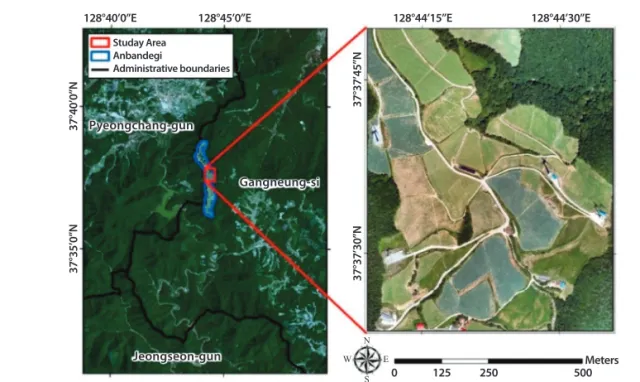
The study area is a part of Anbandegi, which is one of three major cultivation areas of highland Kimchi cabbage in Korea (Fig. 1). As Kimchi cabbage is sensitive to weather conditions and cannot be grown at high temperatures, it is cultivated mainly on the highlands of Kangwon Province, Korea in summer (Kwak and Park, 2019). In addition to highland Kimchi cabbage, cabbage and potato are grown in the study area, and several fallow parcels are also present in the region.

Multitemporal UAV images are used for crop classification because the study area consists of small- scale parcels, and the data acquisition of time-series UAV images covering the entire growth cycles of crops is much easier than that of satellite or aerial photo images. Three-channel UAV images including blue, green, and red spectral channels were acquired in 2018 using a fixed-wing unmanned aerial system (eBee,

senseFly, Switzerland) with a Canon IXUS/ELPH camera. These three visible spectral channels were used for crop classification because the blue channel provides sufficient information to discriminate the different crop types without near-infrared channel (Kwak et al., 2019). For the UAV image acquisition, the forward and side overlaps were set to be 75% and 60%, respectively. Radiometrically corrected ortho- mosaic images were generated using Pix4Dmapper software (Pix4D, Switzerland), taking into account exterior orientation parameters and incoming sunlight information. Finally, nine multitemporal UAV images

Fig. 1. Location map of the study area with UAV imagery acquired on August 15, 2018.

Studay Area Anbandegi

Administrative boundaries

Pyeongchang-gun

Gangneung-si

Jeongseon-gun

128°40’0”E 128°45’0”E 128°44’15”E 128°44’30”E

0 125 250 500 N

S

W E Meters

37°35’0”N37°40’0”N 37°37’30”N37°37’45”N

Table 1. List of UAV images acquired in the study area

No. Acquisition date

1 June 7, 2018

2 June 16, 2018

3 June 28, 2018

4 July 16, 2018

5 August 1, 2018

6 August 15, 2018

7 September 4, 2018

8 September 19, 2018

9 October 13, 2018

(4)

with a spatial resolution of 50 cm are used as inputs for classification experiments (Table 1).

Four classes, including three types of crops and fallow, are considered for supervised classification. A ground truth map based on field surveys was used to select training and test datasets for model training and evaluation, respectively. To ensure spatial independence between training and test datasets, all parcels in the study area were first divided into spatially independent training and reference groups and the proportions of the two groups were 25% and 75%, respectively. Then, training pixels were randomly selected within each training parcel by considering the proportion of each crop parcel in the study area (Table 2). A total of 5,000 training samples were selected based on our previous study (Kwak et al., 2019). For the evaluation of the classification results, all the pixels within the test parcels were used to assess the classification performance of the different LSTM models.

3. Classification Methods 1) Long Short-Term Memory Model

RNN is an artificial neural network designed for sequential data processing. The key feature of the RNN is to determine the output at a current time step using both the output at a previous time step and the input at a current time step, which is particularly efficient to explicitly account for the sequential data dependency.

The most well-known type of RNN family is the LSTM, which was designed to mitigate the limitation

of the regular RNN, where the long-term dependencies cannot be learned because of the vanishing and exploding gradients (Hochreiter and Schmidhuber, 1997). The LSTM unit has important internal functions, including states and gates (Fig. 2). The forget gate (f

t

) first decides whether to remember or forget the information at a previous time step and the input gate (i

t

) then regulates how much of the information at a current time step needs to be maintained. The current cell state is determined by updating the previous cell state using the outputs of the forget and input gates. The output gate (o

t

) controls which part of the current cell state determines the hidden state. Finally, both the cell and hidden states controlled through three different gates are forwarded to the next time step. The computation of the outputs of gates and states can be respectively formulated as:

i

t

= σ (W

ix

x

t

+ W

ih

h

t-1

+ b

i

) (1) f

t

= σ (W

fx

x

t

+ W

fh

h

t-1

+ b

f

) (2) c

t

= f

t

·  c

t-1

+ i

t

 · tanh (W

cx

x

t

+ W

ch

h

t-1

+ b

c

) (3) o

t

= σ (W

ox

x

t

+ W

oh

h

t-1

+ b

o

) (4) h

t

= o

t

·  tanh (c

t

) (5) where W

_*x

and W

_*h

are the weight of a hidden-input gate matrix and an input-output gate matrix, respectively. b

_*

is a bias variable and x

t

is a model input at time t. ^ · denotes an elementwise Hadamard product operator.

σ and tanh are the sigmoid and hyperbolic tangent functions, respectively.

Table 2. Number of training and test pixels for each class Class Training data Test data Highland Kimchi cabbage 2,550 419,119

Cabbage 1,050 168,508

Potato 600 99,690

Fallow 800 134,198

Total 5,000 821,515

Fig. 2. Basic structure of the LSTM unit (modified from Rußwurm and Körner (2018)).

c

t–1 (Cell state)

h

t–1 (hidden state)

c

t

h

t

x

t

σ σ

σ

tanh

tanh input

forget gate

gate output

gate

(5)

The LSTM described above is a network that can solve forward sequence learning problems. However, information on the growth cycle of crops is temporally interrelated from sowing to harvesting in both forward and backward directions (Kwak et al., 2019). Therefore, Bi-LSTM that models sequential data using information from both previous and future time steps could be a promising model for crop classification with multitemporal remote sensing images.

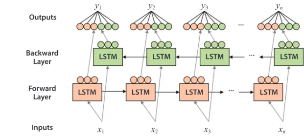
Bi-LSTM combines two independent LSTM architectures where forward and backward information is learned (Fig. 3). For example, the LSTM unit at the second time step outputs the hidden state by concatenating information learned both in the forward direction from the first time step to the second time step and in the backward direction from the last time step to the second time step.

2) LSTM Model Construction

The optimal structures of three different LSTM models, the forward LSTM (F-LSTM), backward LSTM (B-LSTM), and Bi-LSTM are constructed for crop classification in the study area based on preliminary experiments (Table 3). The model structures including a stack of three LSTM layers are employed because LSTM with a multi-layer structure can learn non-linear temporal dependencies (Ienco et al., 2017). The LSTM

model has 64 channels and includes dropout with a rate of 40% for each layer. Dropout is a regularization method that randomly removes some neurons to avoid dependency on specific neurons while training a model (Srivastava et al., 2014). Finally, the fully connected layer with a softmax activation function is stacked on the last LSTM unit to perform the classification. The outputs of the fully connected layer are the probability values summing to one, and the class with a maximum probability value is assigned as a classification result at each pixel. For the analysis of time-series classification results, a many-to-many mode, which returns the output at a final time step, is adopted to produce the classification result at each time step.

To train the LSTM models, categorical cross entropy is applied as a loss function for training the LSTM Fig. 3. Basic structure of the Bi-LSTM model.

y

1

y

²

y

³

y

ⁿ

x

1

x

2

x

3

x

n

LSTM LSTM LSTM LSTM

LSTM Outputs

Backward Layer

Forward Layer

Inputs

LSTM LSTM LSTM

Table 3. Parameters of LSTM models applied in this study:

t and c denote the numbers of inputs used and classes, respectively

Layer Number of channels

Number of parameters Unidirectional

LSTM Bidirectional LSTM

LSTM

t × 64

17,664 35,328

LSTM

t × 64

33,024 98,816

LSTM

t × 64

33,024 98,816

Softmax

t × c

260 516

Total trainable parameters of unidirectional LSTM: 83,972

Total trainable parameters of bidirectional LSTM: 233,476

(6)

architectures, and the Adam optimizer with a learning rate of 1×10

^-4

is also adopted for the optimization of the loss function. The LSTM network is trained over 50 epochs and the training process is stopped early to prevent both overfitting and underfitting of the model when the training loss no longer decreases. The model at the early stopped epoch is defined as the optimal model. All the classification experiments using LSTM were implemented using the Keras Python library (Chollet, 2015).

As any deep learning model has stochastic characteristics, classification using the LSTM models is implemented five times. Averages of five overall accuracy and class-wise accuracy values are used for quantitative measures of the classification performance.

One classification result with the highest overall accuracy is also used for visual comparison with the test data. Non-crop areas are finally masked out to generate crop maps for the study area.

3) Experiment Design

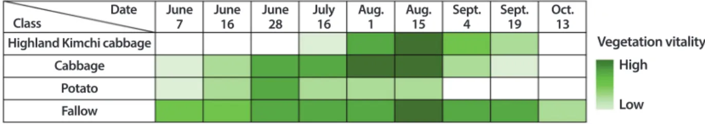
As the focus of this case study is comparing the classification performance of Bi-LSTM with that of unidirectional LSTM, different combinations of input images are first generated and then used for a comparison study. Prior to the classification experiments, the growth cycle stages of crops in the study area based on field surveys was first analyzed to select UAV images useful for crop discrimination (Fig. 4). As shown in Fig. 4, the sowing times of both potato and cabbage are similar (early June), but potato is harvested faster than cabbage (mid-August). The highland Kimchi cabbage is sowed later than potato and cabbage and

harvested in mid-September, similar to cabbage. Two images acquired on June 28 and July 16 provide useful information to identify highland Kimchi cabbage from cabbage because the difference in vegetation vitality between the two crops is large in the two images. In August, highland Kimchi cabbage and cabbage has the highest vegetation vitality, and the difference in vegetation vitality between the two crops and the potato is high. Thus, the images obtained in August are useful for identifying potato. However, it might be difficult to discern crops that have reached the peak of vegetation vitality from fallow with consistently high vegetation vitality. Therefore, it is necessary to collect a time-series image set that can account for the phenological characteristics of all the crops in the study area. As described in the Introduction, however, it is often difficult to construct a full set of time-series images.

From an operational viewpoint, it is necessary to select an optimal LSTM architecture that can achieve satisfactory classification performance even when the acquisition of a full or optimal set of time-series images is difficult.

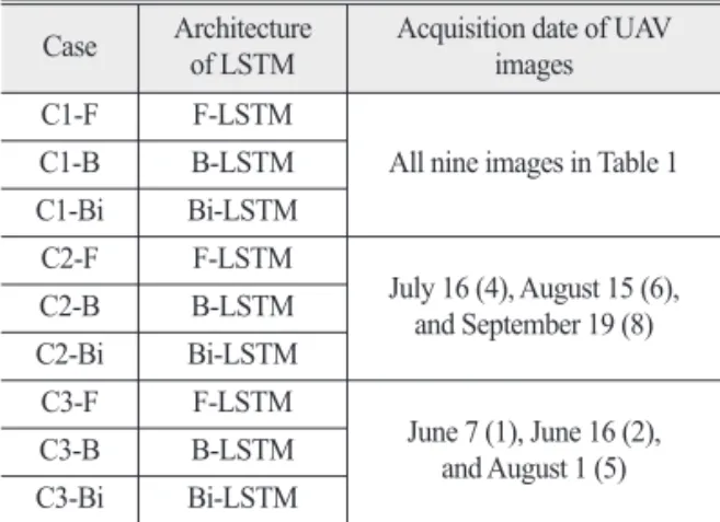
Three representative cases for input image combinations are defined by considering the conditions for UAV image acquisition and the growth cycles of crop classes in the study area: (1) Nine time-series UAV images covering the entire growth cycle of the major crops (C1), (2) Three multitemporal UAV images with information for clear distinctions of major crops (C2), and (3) Three multitemporal UAV images, including images acquired at the seeding stage of crops (C3).

Case C3 represents the case where the distinction between crops is unclear. By considering three different

Fig. 4. Vegetation vitality and growth cycles of crops in the study area based on field surveys.

June 7 Highland Kimchi cabbage

Cabbage Potato Fallow

Date Class

June 16

June 28

July 16

Aug.

1 Aug.

15 Sept.

4 Sept.

19 Oct.

13 Vegetation vitality High

Low

(7)

LSTM model architectures including the F-LSTM, B- LSTM, and Bi-LSTM, a total of nine different cases are tested for comparison purposes (Table 4).

4. Results and Discussion

Fig. 5 presents the average overall accuracy values for nine combination cases of different input images and architectures of the LSTM. Regardless of different combinations of input images, Bi-LSTM outperformed the other unidirectional LSTM architectures. Particularly, Bi-LSTM yielded the smallest variation in overall

accuracy for five repetitions, thereby indicating the most stable LSTM architecture in terms of classification accuracy. When comparing the classification results with respect to different combinations of input images, the LSTM with C1 exhibited the best classification accuracy, regardless of the architecture of the LSTM, but the difference in overall accuracy between the different architectures of LSTM was not significant.

This result is attributed to the rich temporal information from a full time-series dataset covering the entire growth cycle of major crops. In the classification for C2, the accuracy of Bi-LSTM outperformed the other LSTM models by more than 3.4%p. Compared with C1, the classification performance of the Bi-LSTM with C2 was similar to that of the Bi-LSTM with C1 (96.8%

vs. 97.6%), whereas the classification performance of both F-LSTM and B-LSTM decreased. A significant decrease in overall accuracy was observed when C3 was used for classification. However, Bi-LSTM exhibited the highest overall accuracy, with an improvement of approximately 6%p over the F-LSTM. The F-LSTM showed more variations in overall accuracy among the five repetitions, indicating the instability of the LSTM architecture. The highest classification accuracy of Bi-LSTM demonstrates its superiority over the unidirectional LSTM even when images cannot be acquired during the growing period of major crops.

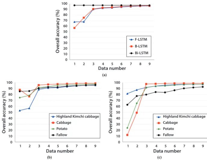
For the interpretations of the superiority of Bi-LSTM over the two unidirectional LSTM architectures, temporal variations of classification results and classification accuracy for C1 were further analyzed by generating nine time-series crop maps (Fig. 6 and Fig. 7). The growing cycle states of crops in the study area in Fig. 4 were also used to interpret the time-series classification results. As shown in Fig. 6 and Fig. 7(a), the classification results on the first date of F-LSTM showed distinctive classification patterns, compared with that of the B-LSTM. As the first date for B-LSTM is October 13, all the crops in the study area were already harvested, thereby yielding many misclassified pixels and the Table 4. Nine combination cases with different input UAV

images and LSTM architectures. The number in parenthesis indicates the data number in Table 1 Case Architecture

of LSTM Acquisition date of UAV images

C1-F F-LSTM

All nine images in Table 1

C1-B B-LSTM

C1-Bi Bi-LSTM

C2-F F-LSTM

July 16 (4), August 15 (6), and September 19 (8)

C2-B B-LSTM

C2-Bi Bi-LSTM

C3-F F-LSTM

June 7 (1), June 16 (2), and August 1 (5)

C3-B B-LSTM

C3-Bi Bi-LSTM

Fig. 5. Average overall accuracy of classification results for nine combination cases with different input images and architectures of LSTM. Vertical lines represent one standard deviation of five overall accuracy values.

100 95 90 85 80 75 70 65 60

F-LSTM B-LSTM Bi-LSTM

C1 C2 C3

Combination case

O v e ra ll a cc u ra c y ( % )

(8)

Fig. 6. Time-series classification maps of both F-LSTM and B-LSTM with a many-to-many method for C1. The number below each classification map indicates the data number in Table 1. The data number of B-LSTM is the reverse of the actual data number.

1 2 3 9

Ground Truth

Highland Kimchi cabbage Cabbage Potato Fallow

Fig. 7. Variations in classification accuracy with respect to each date: (a) overall accuracy, (b) class-wise accuracy of F-LSTM, and (c) class-wise accuracy of B-LSTM. The data number of B-LSTM is the reverse of the actual data number.

(a)

(b)

Data number

100 90 80 70 60 50 40 30 20 10 0

100 90 80 70 60 50 40 30 20 10 0 100

90 80 70 60 50 40 30 20 10 0

1 2 3 4 5 6 7 8 9

1 2 3 4 5 6 7 8 9 1 2 3 4 5 6 7 8 9 Highland Kimchi cabbage

Cabbage Potato Fallow

Highland Kimchi cabbage Cabbage

Potato Fallow F-LSTM

B-LSTM Bi-LSTM

Data number Data number

(c)

O v e ra ll a cc u ra c y ( % )

F -L S T M B -L S T M O v e ra ll a cc u ra c y ( % )

O v e ra ll a cc u ra c y ( % )

(9)

poorest classification accuracy. The classification accuracies of both the unidirectional architectures were improved significantly from the third date (i.e., June 28 for F-LSTM and September 4 for B-LSTM) by including temporal information sufficient to discriminate four classes. The information contained in each date image is sequentially stacked in the unidirectional LSTM, and all the stacked information is reflected in the classification result. In contrast, as shown in Fig.

7(a), the Bi-LSTM yielded the highest classification accuracy for each date by using both forward and backward state information learned at each date during the classification.

The class-wise accuracy presented in Fig. 7(b) and Fig. 7(c) confirms the ability of LSTM to efficiently model the temporal correlation information. The first date in F-LSTM in Fig. 7(b) is a stage where sowing was begun in some crop parcels, but most parcels included bare soils. Consequently, highland Kimchi cabbage was misclassified as cabbage due to mixed crops in the crop parcels with bare soils, thereby yielding low classification accuracy. Moreover, on the first date in B-LSTM in Fig. 7(c) where all the crops have been harvested, crop parcels, except for fallow, were misclassified as highland Kimchi cabbage, leading to the low classification accuracy of cabbage

and potato. However, the classification accuracies of the two unidirectional LSTM architectures were improved substantially whenever temporal information after the first date was transferred to the next time step.

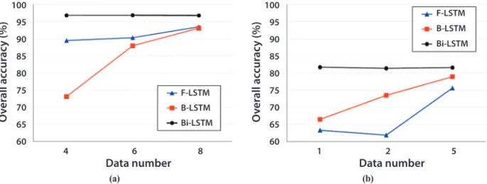
Fig. 8 presents the variations in overall accuracy for C2 and C3. The highest accuracy and the smallest variation of accuracy of Bi-LSTM for both C2 and C3 demonstrate the superiority of Bi-LSTM over the unidirectional LSTM. As shown in Fig. 8(a), the classification accuracy of B-LSTM for C2, which used the September image where cabbage and potato were harvested as the first data, decreased significantly compared to the other LSTM architectures. In addition, the classification accuracy of F-LSTM for C3 was also low until the second date because only information from the sowing stage was used for the F-LSTM (Fig. 8(b)). When considering the variations in the classification accuracy of both F-LSTM and B-LSTM with respect to the input image combination, the classification accuracy of unidirectional LSTM depends heavily on the information content contained in an input image at the beginning date. That is, the higher the classification accuracy on the first date, the higher the classification accuracy of the final classification result.

Particularly, this result is clearly shown for C3, where input images failed to provide sufficient information to

Fig. 8. Variations in overall accuracy for (a) C2 and (b) C3. The data number of B-LSTM is the reverse of the actual data number.

(a)

Data number

4 6 8 1 2 5 100

95 90 85 80 75 70 65 60

F-LSTM B-LSTM Bi-LSTM

100 95 90 85 80 75 70 65 60

Data number (b)

O v e ra ll a cc u ra c y ( % ) O v e ra ll a cc u ra c y ( % )

(10)

discriminate the types of crops. However, the Bi-LSTM always exhibited better classification performance than the unidirectional LSTM from the beginning date because of its ability to fully utilize the information from both previous and future time steps in all directions.

These results confirm the effectiveness of Bi-LSTM in crop classification when limited input images are be used for classification.

5. Conclusion

In this study, the potential of Bi-LSTM for crop classification with multitemporal remote sensing images was investigated. The benefits of using temporal information in forward and backward states by Bi-LSTM were analyzed particularly for the case where either a full set or an optimal set of time-series images covering almost the entire growth cycle of crops is not available, which is often encountered for crop classification using remote sensing images. A case study of crop classification in highland Kimchi cabbage cultivation areas with time-series UAV images demonstrated the superiority of Bi-LSTM over the conventional unidirectional LSTM, regardless of input image combinations. The classification accuracy of Bi-LSTM was greatly improved in the case where some images acquired at a time when discrimination between crops was not apparent were used as inputs for crop classification. The classification performance of unidirectional LSTM was significantly affected by the classification results of the beginning date. In contrast, Bi-LSTM could mitigate the dependency on initial classification results because of its architecture that can consider temporal information in both forward and backward states. However, these results were obtained from a case study with specific crop types. Thus, more experiments should be conducted on other crop areas where the growth cycles are different from those of crops in the study area to comprehensively verify the

efficiency of Bi-LSTM for crop classification with limited input images.

Acknowledgements

This work was carried out with the support of

“Cooperative Research Program for Agriculture Science & Technology Development (Project No.

PJ01350004)” Rural Development Administration, Republic of Korea.

References

Ban, H.-Y., K. S. Kim, N.-W. Park, and B.-W. Lee, 2017. Using MODIS data to predict regional corn yields, Remote Sensing, 9(1): 16.

Chollet, F., 2015. Keras, https://github.com/fchollet/

keras, Accessed on Jul. 13, 2020.

Guidici, D. and M. L. Clark, 2017. One-dimensional convolutional neural network land-cover classification of multi-seasonal hyperspectral imagery in the San Francisco Bay area, California, Remote Sensing, 9(6): 629.

Hochreiter, S. and J. Schmidhuber, 1997. Long short- term memory, Neural Computation, 9(8):

1735-1780.

Ienco, D., R. Gaetano, C. Dupaquier, and P. Maurel, 2017. Land cover classification via multitemporal spatial data by deep recurrent neural networks, IEEE Geoscience and Remote Sensing Letters, 14(10): 1685-1689.

Kim, Y., N.-W. Park, and K.-D. Lee, 2017. Self- learning based land-cover classification using sequential class patterns from past land-cover maps, Remote Sensing, 9(9): 921.

Kwak, G.-H. and N.-W. Park, 2019. Impact of texture

information on crop classification with machine

learning and UAV images, Applied Sciences,

(11)

9(4): 643.

Kwak, G.-H., M.-G. Park, C.-W. Park, K.-D. Lee, S.-I. Na, H.-Y. Ahn, and N.-W. Park, 2019.

Combining 2D CNN and bidirectional LSTM to consider spatio-temporal features in crop classification, Korean Journal of Remote Sensing, 35(5): 681-692 (in Korean with English abstract).

Lee, J., B. Seo, and S. Kang, 2017. Development of a biophysical rice yield model using all- weather climate data, Korean Journal of Remote Sensing, 33(5-2): 721-732 (in Korean with English abstract).

Liu, G. and J. Guo, 2019. Bidirectional LSTM with attention mechanism and convolutional layer for text classification, Neurocomputing, 337:

325-338.

Mou, L., P. Ghamisi, and X. X. Zhu, 2017. Deep recurrent neural networks for hyperspectral image classification, IEEE Transactions on Geoscience and Remote Sensing, 55(7): 3639- 3655.

Na, S.-I., C.-W. Park, K.-H. So, J.-M. Park, and K.-D.

Lee, 2017. Satellite imagery based winter crop classification mapping using hierarchical Classification, Korean Journal of Remote Sensing, 33(5): 677-687 (in Korean with English abstract).

Na, S.-I., C.-W. Park, K.-H. So, H.-Y. Ahn, and K.-D.

Lee, 2018. Application method of unmanned aerial vehicle for crop monitoring in Korea, Korean Journal of Remote Sensing, 34(5-2):

829-846 (in Korean with English abstract).

Rußwurm, M. and M. Körner, 2018. Multi-temporal

land cover classification with sequential recurrent encoders, ISPRS International Journal of Geo- Information, 7(4): 129.

Schuster, M. and K. K. Paliwal, 1997. Bidirectional recurrent neural networks, IEEE Transactions on Signal Processing, 45(11): 2673-2681.

Sonobe, R., Y. Yamaya, H. Tani, X. Wang, N. Kobayashi, and K.-I. Mochizuki, 2017. Mapping crop cover using multi-temporal Landsat 8 OLI imagery, International Journal of Remote Sensing, 38(15): 4348-4361.

Srivastava, N., G. Hinton, A. Krizhevsky, I. Sutskever, and R. Salakhutdinov, 2014. Dropout: A simple way to prevent neural networks from overfitting, Journal of Machine Learning Research, 15(1):

1929-1958.

Sun, Z., L. Di, and H. Fang, 2019. Using long short- term memory recurrent neural network in land cover classification on Landsat and Cropland data layer time series, International Journal of Remote Sensing, 40(2): 593-614.

Yang, L., Y. Li, J. Wang, and Z. Tang, 2019. Post text processing of Chinese speech recognition based on bidirectional LSTM networks and CRF, Electronics, 8(11): 1248.