On the Modified Supplementary Variable Technique for a Discrete-Time GI/G/1 Queue with Multiple Vacations
Doo Ho Lee
†*Department of Industrial and Management Engineering, Kangwon National University
복수휴가형 이산시간 GI/G/1 대기체계에 대한 수정부가변수법
이 두 호
강원대학교 산업경영공학과
This work suggests a new analysis approach for a discrete-time GI/G/1 queue with multiple vacations. The method used is called a modified supplementary variable technique and our result is an exact transform-free expression for the steady state queue length distribution. Utilizing this result, we propose a simple two-moment approximation for the queue length distribution. From this, approximations for the mean queue length and the probabilities of the number of customers in the system are also obtained. To evaluate the approximations, we conduct numerical experiments which show that our approximations are remarkably simple yet provide fairly good performance, especially for a Bernoulli arrival process.
Keywords: Modified Supplementary Variable Technique, Discrete-Time Queue, Queue Length Distribution, Multiple Vacations, Two-Moment Approximation
1. Introduction
Most real queueing situations arising in banks, computer net- works, telecommunication systems, manufacturing systems, etc. can be modeled as queueing systems with general inter- arrival times and general service times. These queueing sys- tems present an interest subject for which to devise a practical analysis method. However, due to the limited information on their distributions, the analysis of such a queue is notoriously difficult. While several approximations have been proposed, they are often computationally demanding. Moreover, most of the approximation methods have been applied to conti- nuous- time queueing systems.
Thanks to recent advances in computer and telecommuni- cation technology, the importance of discrete-time queueing
systems has been increased. That is why continuous-time queueing systems can not accurately give the performance measures of computer and telecommunication systems where basic operational units are bits, packets and cells, although they have been used in the past to approximately evaluate some performance measures of these systems. Hence, discrete-time queueing systems are potentially more suitable for applica- tion to the digital computer and communication networks.
In discrete-time queueing systems, the time axis is segmen- ted into a sequence of equal intervals of unit duration, called slots. It is always assumed that interarrival times, service times, and vacation times are integral multiples of a slot duration. Also, it is assumed that the state of the system changes only at a slot boundary
⋯. Under these assumptions, note that an arrival and a departure can occur simultaneously at a slot boundary. Considering the order of
†Corresponding author : Professor Doo Ho Lee, Department of Industrial and Management Engineering, Kangwon National University, Samcheok 25913, Korea, Tel : +82-33-570-6583, Fax : +82-33-570-6589, E-mail : [email protected] Received March 10, 2016; Revision Received July 17, 2016; Accepted July 17, 2016.
these simultaneous events, there have been two typical as- sumptions: late arrival system (LAS) and early arrival system (EAS). According to the LAS model, a potential arrival takes place in the interval
and a service completion occurs in the interval
, where
and
represent lim
→
and lim
→ , respectively. On the other hand, a potential arrival takes place in the interval
and a service completion occurs in the interval
under the EAS model. For more details, see Hunter (1983) and Bruneel and Kim (1993)
The conventional supplementary variable technique (SVT) is known to be originated by Cox (1955), and has become one of the most frequently used approaches for both the con- tinuous and discrete-time queuing systems. The method we use in the present work is a modified SVT, where the last step of the modified SVT is different from that of the con- ventional SVT. The first step is to define a Markov chain by including appropriate supplementary variables into the state vector. The second step is to construct the steady state sys- tem equations. The last step is to solve these equations. The last step of the conventional SVT is to obtain the probability generating functions (PGFs) of the number of customers in the system/queue by solving the system equations in the transform domain. On the other hand, the last step of the modified SVT is to directly sum each equation after multi- plying a supplement variate. The result thus obtained is the steady state queue length distribution not expressed as the form of transformation but in terms of conditional expecta- tions. In other words, we derive an exact transform-free ex- pression for the steady state queue length distribution. This method is illustrated by the GI/G/1 queue with multiple vaca- tions (for more definitions, see the following sections).
There have been several studies on the discrete-time queue with general interarrival times and general service times. For the standard GI/G/1 queue, see Murata and Miyahara (1991), who obtain the waiting time distribution under the assump- tion that PFGs of the sojourn time distributions are repre- sented as rational polynomials. Chaudhry (1993) also obtains closed-form expressions of waiting time distributions via a root-finding method. For the batch arrival GI
X/G/1 queue, Chaudhry and Gupta (2001) present a procedure for comput- ing waiting time probabilities and its PGF by analyzing the PGF of the unfinished work. For the finite waiting spaces queue, Haβlinger (1995) and Linwong et al. (2004) analyze the queue length distributions for the GI/G/1/K and GI
X/G/
1/K queue, respectively. They use a polynomial factorization approach. The restriction of their approach is that the inter- arrival time distribution, service time distribution, and batch size distribution should all be of finite support. For the in- finite server GI/G/∞ queue, Eliazar (2008) analyzes the out- put process and the queue process making use of the stat- istical properties of the stochastic maps. The studies noted above are based on the transformation technique. As a con- sequence, all their results are expressed as the transformed terms.
Addressing a continuous-time queue, Chae et al. (2004) present the transform-free queue length distribution for the GI/G/1/K queue with multiple vacations. They propose ob- taining the queue length distribution by using the modified SVT. However, to the best of the author’s knowledge, there have been only one report on utilizing the modified SVT for the discrete-time queue. Chae et al. (2008) first apply the modified supplementary variable technique to the discrete- time GI/G/1/K queue without vacations. The purpose of this paper is to extend the work of Chae et al. (2008) considering not finite buffer but multiple vacations. In other words, this work shows the modified SVT for discrete-time queues with general interarrival times, general service times, and general vacation times.
The remainder of this paper is organized as follows. In Section 2, we analyze the queue length distribution of the discrete-time GI/G/1 queue with multiple vacations. In Section 3, we propose a simple approximation, called a two-moment approximation, for the queue length distribution. The two- moment approximation for the continuous-time queue has been reported in the literatures Kim and Chae (2003) and Choi et al. (2005), but there is no precedent for the discrete- time queue. Numerical experiments are conducted to demon- strate that our approximations are remarkably simple yet pro- vide fairly good performance, especially for a Bernoulli ar- rival process.
2. The Steady State Queue Length Distribution of a GI/G/1 Queue with Multiple Vacations
In this section, we derive a transform-free distribution of the steady state queue length in the LAS of the GI/G/1/MV queue, where MV stands for multiple vacations. In the multiple va- cations model, the server leaves for a vacation if there is no customer to serve in the system at the end of a service. If the server returns from a vacation finding the system nonempty, it begins to serve the customers and continues serving until the system becomes empty again. If the server returns from a vacation finding the system empty, it leaves for another vaca- tion, and repeats vacations in this manner until it returns from a vacation finding the system nonempty (see Takagi (1993)).
Just like a service, a vacation is assumed to end in
and immediately after the arrival of a customer and to begin in
and immediately after a service completion. We fur- ther assume that customers leave the system on a first-in first- out basis. Interarrival times, service times, and vacation times are independent and identically distributed random variables (R.V.s) denoted by the generic R.V.s A, S, and V, respectively.
Consider the Markov chain
⋯
, where
denotes the number of customers
in the system at
and the supplementary variables
,
, and
respectively denote the remaining inter- arrival time, the remaining service time, and the remaining vacation time all at
. We define the probability mass func- tions as follows:
⋯,
⋯,
⋯,
lim
→∞
,
≥ ⋯,
lim
→∞
≥ ⋯.
Let
∞,
∞, and
∞denote the sequences of interarrival times, service times, and vacation times and they are mutually independent. By considering mutually ex- clusive events that can occur during one slot, we construct the steady state system equations as follows :
≥
(1a)
≥
(1b)
Due to
, one less equation is required. The left- hand sides of (1) represent the probabilities of the system state at
in a steady state. The right-hand sides of (1) are then expressed in terms of the probabilities of the system state at
in a steady state, together with the probabilities of all potential queueing activities that can happen during
. Notice that (1) is the difference equations, which corre- spond to the differential equations in the continuous-time queue.
Remark 1 :
is the joint probability of three events when the server is busy (on vacation) in a steady state.
One event is that the number of customers in the system is n at
. Another event is that service (vacation) completion oc- curs in
due to
. The other event is that arrival takes place in
due to
.
In the modified SVT, we first sum (1a), both over i and j,
≤ ≤ ∞
and sum (1b) both over i and k,
≤ ≤ ∞. Then, we multiply i+1 to both sides of (1) and sum over i, j, and k,
≤ ≤ ∞. Finally, we multiply j+1 to both sides of (1a) and sum both over i and j,
≤ ≤ ∞, and then multiply k+1 to both sides of (1b) and sum both over i and k,
≤ ≤ ∞
.
Now, we apply above procedure to the model. We first sum (1a), both over i and j,
≤ ≤ ∞, and sum (1b) both
over i and k,
≤ ≤ ∞. Simplifying the results (for more details, see Appendix A), we obtain
∞
∞
∞
≥ , (2a)
∞
∞
∞
≥ . (2b) In order to express (2) in terms of meaningful quantities, let
and
denote the probability that an arriving cu- stomer sees n customers when the server is on vacation and when the server is busy, respectively. Likewise, let
de- note the probability that a departing customer leaves behind n customers. Note that
. We verify that the arrival rate and departure rate are
and a stable system satisfies
.
Based on the assumption mentioned above, expressing (2) in terms of
,
, and
leads to
≥ , (3) which is known as the Burke’s theorem.
In order to express the results of the next procedure, we de- fine the following probabilities and conditional expectations for
≥ :
∞
∞
,
∞
∞
,
,
,
,
, and
, where
is the remaining service time (vacation time) at the arrival epoch of a customer who sees n customers in the sys- tem and
is the remaining interarrival time at the departure epoch of a customer who leaves behind n custom- ers in the system (at the epoch when the server completes its vacations, finding n customers in the system). Here,
and
.
Next, we multiply i+1 to both sides of (1a) and sum over i and j,
≤ ≤ ∞. Simplifying the results (for more de- tails, see Appendix B), we obtain
∞
∞
∞
≥
(4)
On the other hand, we multiply j+1 to both sides of (1a) and sum over i and j,
≤ ≤ ∞. Simplifying the results, we obtain
∞
∞
∞
∞
∞
≥
(5)
Remark 2 :
∞
∞
in (5) means the rate that the server takes vacations. By multiplying the ex- pected length of a vacation time,
∞
∞
becomes the long-run proportion of time the server is on vacation. Since
is not only the traffic intensity but also the long-run proportion of time that the server is busy,
becomes the long-run proportion of time that the server is on vacation.
Now, we want to express (4) and (5) in terms of identities
,
, and
. For this, we introduce the next lemma : Lemma 1 : In a steady state, the following relations hold :
∞
,
≥ ,
∞
,
≥ ,
∞
,
≥ ,
and
∞
,
≥ .
Proof : See Appendix C.
By utilizing the results of Lemma 1, we obtain the queue length equations of the GI/G/1/MV when the server is on va- cation as follows :
Theorem 1 : The queue length distribution for GI/G/1/MV when the server is on vacation satisfies the following simul- taneous equations:
≥
(6)
≥ (7)
Proof.
∞
is the rate (or the expected frequency per unit time) that an arriving customer sees n customers when the server is on vacation. Since
is the expected num- ber of arrivals per unit time and
is the probability that an arriving customer sees n customers when the server is on vacation, we have the concrete result :
∞
. In addition,
∞
is the rate that a departing customer leaves behind n customers in the sys- tem. Since
is also the expected number of departures per unit time and
is the probability that a departing customer leaves behind n customers in the system,
∞
should hold. Using Lemma 1, we can re- write the results of (4) and (5) as (6) and (7).
We then have the following transform-free expressions for the queue length distribution just before an arrival and at an
arbitrary epoch when the server is on vacation, all in product forms.
Theorem 2 : The steady state queue length distribution for GI/G/1/MV when the server is on vacation is given by
≥
(8)
≥
(9)
where
,
, and
.
Proof : For each n, solving (6) and (7) simultaneously leads to (8). Finally, (9) is derived by combining (8) with either (6) or (7).
Note that (8) is a similar form of the steady state queue length distribution of the birth and death process (see Wolff (1989)). The procedure of obtaining
and
is the same. Multiplying i+1 to both sides of (1b) and summing over i and k,
≤ ≤ ∞, we have
∞
∞
∞
∞
∞
∞
∞
≥
(10) Multiplying k+1 to both sides of (1b) and summing over i and k,
≤ ≤ ∞, we have
∞
∞
∞
∞
∞
∞
∞
≥
(11)
Expressing (10) and (11) by using Lemma 1, we obtain the queue length equations of the GI/G/1/MV when the server is busy as follows :
Theorem 3 : The queue length distribution for GI/G/1/MV when the server is busy satisfies the following simultaneous equations :
(12)
≥
(13)
≥ .
Proof : To simplify (10) and (11) meaningfully, we use the relations
∞
and then, we obtain (12) and (13).
∞
is the rate that an arriving custom- er sees n customers when the server is busy servicing. Since
is the expected number of arrivals per unit time and
is the probability that an arriving customer sees n customers when the server is busy, we have the concrete result :
∞
. Using Lemma 1 and the fact that
∞
, we can rewrite the results of (10) and (11) as (12) and (13), respectively.
We finally have the following transform-free expressions for the queue length distribution just before an arrival and at an arbitrary epoch when the server is busy, all in product forms.
Theorem 4 : The steady state queue length distribution for GI/G/1/MV when the server is busy is given by
≥ , (14)
≥ , (15) where
,
,
×
,
, and
.
Proof : For each n, solving (12) and (13) simultaneously leads to (14). Finally, (15) is derived by combining (14) with either (12) or (13).
Our results above are expressed in terms of
,
,
, and
, which are all conditional expectations of supple- mentary variables. In general, they are not easy to compute,
except for some special cases such as Bernoulli arrival, geo- metric service times, or geometric vacation times. However, the availability of such expressions provides a basic idea for developing approximations for various performance meas- ures of practical interest, which will be discussed in the fol- lowing sections.
Remark 3 : These transform-free expressions for the discrete- time queues are not available in previous studies, although our method is intuitive and easy to follow. It is interesting to state that (9) and (15) in this work take the same forms as (12) and (18) in Chae et al. (2004) when
→ ∞. Specifi- cally, the definitions of the conditional expectations
and
in this paper are slightly different from those in Chae et al. (2004), because
and
are not defined in the continuous-time queue but have positive probabilities in the discrete-time queue. Nonetheless, (9) and (15) in this work take exactly the same forms as (12) and (18) in Chae et al. (2004).
Remark 4 : Heuristic interpretations for Eqs. (6), (7), (12) and (13) can be found in the Chae et al. (2002). Here, we briefly explain the first equation in (6).
is the time-average probability that there is no customer in the system when the server is on vacation.
is the expected frequency that a departing customer leaves behind the empty system. And,
is the expected remaining interarrival time when the system becomes empty. If the state of the server changes from
“busy” to “on vacation”, there is no customer and the server leaves for vacations at the same time. Therefore,
is the long-run proportion of time that there is no customer in the system when the server is on vacation. Chae et al. (2002) explains the time-average probability of the queue length dis- tribution for the continuous-time GI/G/c/K queue by using the tax collection examples. Nevertheless, we can apply their same interpretations for the queue length distribution to our results.
3. The Two-Moment Approximation for the Queue Length Distribution and Its Performance
Based on the expressions given in Section 2, we now propose a simple two-moment approximation for the steady state queue length distribution through approximation of
,
,
, and
. From this, approximations for several perform-
ance measures can also be obtained. We employ the follow-
ing approximation scheme for
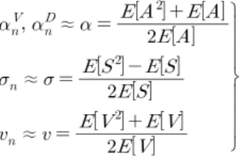
≥ :
≈
≈
≈
(16)
where
is the second moment of any discrete R.V. Y with a distribution function F, and
±
is the mean of the equilibrium distribution of F.
Remark 5 : In our setting, the remaining interarrival time of a customer both at a service completion epoch and at a vaca- tion termination epoch does not contain 0. In contrast, both the remaining service time and the remaining vacation time at a customer arrival epoch contain 0. Therefore, in terms of the discrete-time inspection paradox,
,
,
, and
can approximate
, , and
, respectively.
Applying (16) to (8), (9), (14), and (15), we obtain two- moment approximations for the steady state queue length dis- tribution as follows :
≈
≈
≥
≈
≈
≥
≈
≥
≈
≥
(17)
where
,
,
,
,
,
,
, and
. Note that (16) is exact for the Bernoulli arrival process, geometric service times, and geometric vacation times in the LAS, respectively, due to the memoryless property of the geometric distribution.
Therefore, our approximations in (17) lead to the exact queue length distribution for the Geo/Geo/1/GMV queue, where GMV stands for geometric multiple vacations. Similar ap- proximations to those proposed in (17) have been used to ap- proximate a continuous-time queue by Kim and Chae (2003) and Choi et al. (2005). For some range of parameter values, (17) may result in negative probabilities. In such a case, one can set those approximate values to zero.
From (17), approximations of various mean performance measures can be obtained, such as approximations for the mean numbers of customers in service, in the queue, and in the entire system. Subsequently, approximations for the mean
time a customer spends in the queue and in the system also follow from Little’s formula. Among others, we present the approximate value for the mean of customers in the entire sys- tem, denoted by
. From (6), (7), (12), and (13), we have
∞
∞
, (18)
∞
,
∞
∞
(19)
∞
. Combining (18) and (19) with (16) yields
≈
∞
∞
, (20)
where
and
are approximate values for
and
, respectively.
To evaluate the performance of our approximation, exten- sive numerical experiments have been carried out for a varie- ty of interarrival times, service times, and vacation times, but only a few that exhibit representative information are pre- sented in <Table 1> through <Table 3>. In all cases, exact values are calculated by differentiating the PGFs of each queue length distribution or carrying out simulation experi- ments.
denotes a 2-Negative binomial distribution and
denotes a mixed-geometric distribution of order 2.
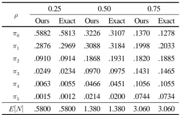
<Table 1> presents results for
and
of several Ber- noulli arrival queues with GMV in low (
) traffic, in moderate (
) traffic, and high (
) traffic, respec- tively. Through our numerical investigations, we have obser- ved that our results closely match the exact results regardless of the traffic intensities. <Table 2> shows results of the case of Bernoulli arrival queues with general multiple vacations.
Interestingly, our approximation functions well even though vacation times do not have geometric distributions.
Table 1.
and
for
queues
0.25 0.50 0.75
Ours Exact Ours Exact Ours Exact
.6818 .6818 .4167 .4167 .1923 .1923
.2514 .2514 .2604 .2604 .2504 .2504
.0544 .0544 .1411 .1411 .1901 .1901
.0102 .0102 .0601 .0601 .1291 .1291
.0018 .0018 .0238 .0238 .0845 .0845
.0003 .0003 .0091 .0091 .0547 .0547
.4000 .4000 .9000 .9000 2.400 2.400
0.25 0.50 0.75
Ours Exact Ours Exact Ours Exact
.6818 .6818 .4167 .4617 .1923 .1923
.2483 .2490 .3204 .3241 .2380 .2443
.0562 .0552 .1532 .1502 .1836 .1826
.0112 .0112 .0652 .0635 .1278 .1248
.0021 .0023 .0266 .0264 .0863 .0838
.0004 .0005 .0107 .0110 .0576 .0563
.4050 .4050 1.030 1.030 2.535 2.535
0.25 0.50 0.75
Ours Exact Ours Exact Ours Exact
.6818 .6818 .4167 .4617 .1923 .1923
.2655 .2645 .3781 .3706 .3258 .3056
.0454 .0471 .1430 .1532 .2193 .2346
.0063 .0059 .0446 .0447 .1244 .1334
.0008 .0006 .0128 .0114 .0665 .0686
.0001 .0001 .0035 .0027 .0347 .0339
.3792 .3792 0.875 0.875 1.838 1.838
Table 2.
and
for
queues
0.25 0.50 0.75
Ours Exact Ours Exact Ours Exact
.5357 .5357 .2778 .2778 .1136 .1136
.2994 .3000 .2908 .2932 .1764 .1801
.1119 .1113 .1958 .1945 .1722 .1728
.0367 .0367 .1135 .1121 .1444 .1431
.0114 .0114 .0609 .0604 .1123 .1106
.0034 .0035 .0313 .0313 .0836 .0821
.7050 .7050 1.630 1.630 3.435 3.435
0.25 0.50 0.75
Ours Exact Ours Exact Ours Exact
.4903 .4963 .2428 .2513 .0966 .1025
.3037 .2982 .2712 .2705 .1565 .1616
.1293 .1266 .1976 .1913 .1606 .1587
.0491 .0494 .1248 .1208 .1415 .1373
.0178 .0186 .0734 .0721 .1154 .1115
.0063 .0069 .0414 .0416 .0897 .0870
.8346 .8346 1.889 1.889 3.824 3.824
0.25 0.50 0.75
Ours Exact Ours Exact Ours Exact
.5882 .5813 .3226 .3107 .1370 .1278
.2876 .2969 .3088 .3184 .1998 .2033
.0910 .0914 .1868 .1931 .1820 .1885
.0249 .0234 .0970 .0975 .1431 .1465
.0063 .0055 .0466 .0451 .1056 .1055
.0015 .0012 .0214 .0200 .0744 .0734
.5800 .5800 1.380 1.380 3.060 3.060
The results for the non-Bernoulli arrival queues are ap- pended in Table 3. In this case, however, approximations can deteriorate. Thus, one should use the approximations cau- tiously for non-Bernoulli arrival queues. Note that our ap- proximations do not require the whole distributions of A, S, and V, but only the first two moments. The first two mo- ments alone will lead to quick and simple approximate results.
Table 3.
for
queues
0.2 0.4 0.6 0.8
Exact Ours
.3063 .2750
.5977 .5667
1.153 1.150
2.788 2.900
0.2 0.4 0.6 0.8
Exact Ours
.3298 .3583
.7389 .7889
1.596 1.650
4.234 4.233
0.2 0.4 0.6 0.8
Exact Ours
.3022 .2656
.5312 .5167
.8516 .9813
1.823 2.300
0.2 0.4 0.6 0.8
Exact Ours
.3143 .3438
.6261 .7111
1.213 1.388
3.092 3.300
Remark 6 : One may consider
∞ , where
is the
approximate value for
. From (6) and (12),
∞ can
be written as
∞
∞
. For Bernoulli arrival queues,
∞ holds due to
∞
and
∞
. For non-Bernoulli arrival queues,
however,
∞ does not hold. In this case, we ap-
proximate
to
∞ by normalization.
4. Conclusions
This paper aimed at analyzing a discrete-time GI/G/1 queue with multiple vacations and making a two-moment approx- imation of the mean queue length and the probabilities of the number of customers in the system for that queue. To this end, we derived a transform-free steady state queue length distribution,
and
. The transform-free queue length distribution for other vacation models, such as the sin- gle vacation model and set-up time model, can be derived by the modified SVT.
Note again that our approximation is especially useful when distributions of A, S, and V are unknown and have to be estimated, since our methods do not require fitting dis- tributions to sample data but only require that the first two moments be obtained. On this basis, the approximation pro- cedure is simple and quick. We anticipate that our two-mo- ment approximation will be beneficial to those practitioners who seek simple and quick practical answers to queueing systems with multiple vacations.
Finally, it is noted that the modified SVT is basically the same as the conventional SVT except that in the last step of solving system equations. We multiply a supplementary var- iate i+1, j+1, and k+1 and then sum over both i, j, and k. As a result, we obtained the simultaneous equations for the queue length probabilities in terms of conditional expectations of the supplementary variables. We believe that our approach will help the readers better understand discrete-time queue- ing systems and gain new insight into their analyses.
References
Bruneel, H. and Kim, B. G. (1993), Discrete-time models for communication systems including ATM, Kluwer Academic Publishers, New York.
Cox, D. R. (1955), The analysis of non-Markovian stochastic processes by the inclusion of supplementary variables, Mathematical Proceedings of the Cambridge Philosophical Society, 51(3), 433-441.
Chae, K. C., Kim, N. K., and Choi, D. W. (2002), An interpretation of the equations for the GI/GI/c/K queue length distribution, Journal of the Korean Institute of Industrial Engineers, 28(4), 390-396.
Chae, K. C., Kim, N. K., and Yoon, B. K. (2004), On the queue length dis- tribution for the GI/G/1/K/VM queue, Stochastic Analysis and Applica- tions, 22(3), 647-656.
Chae, K. C., Lee, D. H., and Kim, N. K. (2008), On the modified supplementary variable technique for the discrete-time GI/G/1/K queue, Journal of the Korean Operations Research and Management Science Society, 33(1), 107-115.
Chaudhry, M .L. (1993), Alternative numerical solutions of stationary queue- ing-time distribution in discrete-time queues : GI/G/1, Journal of the Operational Research Society, 44(1), 1035-1051.
Chaudhry, M. L. and Gupta, U. C. (2001), Computing waiting-time proba- bilities in the discrete-time queue : GIX/G/1, Performance Evaluation, 43(2/3), 123-131.
Choi, D. W., Kim, N. K., and Chae, K. C. (2005), A two-moment approx- imation for the GI/G/c queue with finite capacity, Informs Journal on Computing, 17(1), 75-81.
Eliazar, I. (2008), On the discrete-time G/GI/∞ queue, Probability in the Engineering and Informational Sciences, 22(4), 557-585.
Hunter, J. J. (1983), Mathematical techniques of applied probability, discrete time models : techniques and applications, Academic Press, New York, 2.
Haβlinger, G. (1995), A polynomial factorization approach to the discrete time GI/G/1/(N) queue size distribution, Performance Evaluation, 23(3), 217-240.
Kim, N. K. and Chae, K. C. (2003), Transform-free analysis of the GI/G/1/K queue through the decomposed Little’s formula, Computers and Opera- tions Research, 30(3), 353-365.
Linwong, P., Kato, N., and Nemoto, Y. (2004), A polynomial factorization approach for the discrete time GIX/G/1/K queue, Methodology And Computing In Applied Probability, 6(3), 277-291.
Murata, M. and Miyahara, H. (1991), An analytic solution of the waiting time distribution for the discrete-time GI/G/1 queue, Performance Evaluation, 13(2), 87-95.
Takagi, H. (1993), Queueing analysis, North-Holland, Amsterdam, 2.
Wolff, R. W. (1989), Stochastic modeling and the theory of queues, Prentice- Hall, New Jersey.