A Non-Linear Exponential(NLINEX) Loss Function in Bayesian Analysis

2004, Vol. 15, No. 4, pp. 899∼910

A Non-Linear Exponential(NLINEX) Loss Function in Bayesian Analysis

A. F. M. Saiful Islam¹⁾․M. K. Roy²⁾․M. Masoom Ali³⁾

Abstract

In this paper we have proposed a new loss function, namely, non-linear exponential(NLINEX) loss function, which is quite asymmetric in nature.

We obtained the Bayes estimator under exponential(LINEX) and squared error(SE) loss functions. Moreover, a numerical comparison among the Bayes estimators of power function distribution under SE, LINEX, and NLINEX loss function have been made.

Keywords : Bayes estimator, Linear exponential(LINEX) loss function, Non-linear exponential(NLINEX) loss function and Square error(SE) loss function.

1 Introduction

In many estimation and prediction problems use of symmetric loss functions may be inappropriate. This has been recognized by Ferguson (1967), Zellner and Geisel (1973), Atchison and Dunmore (1975), Berger (1980), Zellner (1986) and Schabe (1991). Some new loss functions were studied by Rue (1995).

An asymmetric loss function is a model that defines unequal loss to the positive and negative error of the same magnitude. In such a situation Varian (1975), Zellner (1986) proposed a loss function called LINEX loss function. Wahed and Uddin (1998) suggested a loss function, which is a modification of LINEX loss function, known as modified linex (MLINEX) loss function.

The loss function given by Varian (1975), Zellner (1986), Wahed and Uddin (1998) were asymmetric in nature and linear function of the error. In this paper 1) First Author : Department of Statistics, Chittagong University, Chittagong - 4331,

Bangladesh

2) Department of Statistics, Chittagong University, Chittagong - 4331, Bangladesh

3) Department of Statistics, Mathematical Sciences, Ball Stat University, Muncie, IN 47306 USA

we have proposed a new loss function that is asymmetric in nature, and non-linear function of the error called non-linear exponential (NLINEX) loss function. It is also a modification of LINEX loss function but this modification is done in the sense that the asymmetric loss function may not be always linearly related with its exponential form of loss. Such a non-linear loss over the entire distribution may occur in many real life data. So the asymmetric loss function may be non-linearly related with its exponential form of loss which claims the name non-linear exponential (NLINEX) loss function.

2. Proposed NLINEX loss function

If D represents the estimation error in estimating θ by θˆ i.e., D = θˆ - θ, then we introduce the following asymmetric loss function of the form

L( D) = k exp (cD) + γD²- γD - k, r, c > 0 (2.1) But for a loss function we must have, L( D) = 0 when D = 0 i.e., when θˆ - θ and L( D) must be minimum at D = 0. Equation (2.1) satisfies L( D) = 0, at D = 0. For a minimum to exist at D = 0 we must have, L'( D)|_{D = 0}= 0, i.e., ck = γ. Putting ck = γ in (2.1), we obtain the loss function

L( D) = k[exp (cD) + cD²- cD- 1], k > 0 , c > 0, (2.2) which is the required form of non-linear exponential (NLINEX) loss function.

Expression (2.2) is easier to deal with as compared to expression (2.1). Expression (2.2) can be re-written as

L( D) = k[ { exp ( cD) - cD - 1 } + cD²]

= k[LINEX loss function + c{squared error(SE) loss function}].

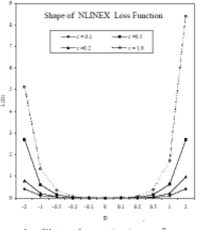
Hence, NLINEX loss function is a linear combination of LINEX loss function and SE loss function. We can expect that this proposed new loss function would preserve the estimation error due to both LINEX and SE form of loss. The following figure shows shape of NLINEX loss function.

For multiparameter estimation problems and multivariate prediction problems there is a need to extend the form (2.2). Let D_i= θˆ - θ_{i i} be the error in estimating θ_i by use of the estimate ˆ. Then the extended NLINEX loss θ_i function is given by,

L( D) = ∑

n

i = 1k_i[ exp (c_iD_i) + c_iD²_i- c_iD_i- 1], (2.3) provided c_i> 0, k_i> 0, i = 1,2,…, n and D' = ( D₁, D₂, …, D_n). This is a convex loss function such that L( 0) = 0, L'( 0) and D = 0 corresponds to a minimum. The function (2.3) can be utilized in multiparameter estimation and prediction problems.

Shape Characteristics of the NLINEX Loss Function:

(i) For c > 0, the function decreases almost nonlinearly when D = θˆ - θ < 0. On the contrary it increases almost nonlinearly when D = θˆ - θ > 0.

Figure 1 : Plots of exp (cD) + cD²- cD - 1

(ii) On expanding exp (cD) by Taylor series expansion when c is small omitting terms of higher order we get, L(D)= c₁D² where c₁= ( c + c²)/2. Thus for small values of c, optimal estimates and predictions under NLINEX loss function are close to the estimates under SE loss function.

(iii) The parameter can be chosen to provide a variety of asymmetric effects.

In the following theorem we shall present the form of Bayes estimator under NLINEX loss function.

3. Theorems

Theorem 3.1 For NLINEX loss function, the Bayes estimator for a parameter θ is

ˆθ

NL = - [ ln E_θ{ exp ( - cθ) } - 2E_θ(θ) ]/( c + 2 ), where, E_θ stands for posterior expectation.

Proof: To proof the theorem a simple assumption is considered as follows.

Assumption: Since Bayes estimator is consistent, hence

n→∞limE( θˆ - θ)^r → 0 , r≥2 . (3.1)

Now let us consider the estimator for a parameter θ relative to the following proposed NLINEX loss function

L( θˆ : θ) = k[ exp {c(θˆ - θ) }

+ c( θˆ - θ)²- c( θˆ - θ)- 1] , k > 0 , c > 0 . (3.2) Again let, p( θ|x) denote the posterior distribution of Θ where p( θ) is assumed to be a prior density with θ ∈ Ω, the parameter space. Then the posterior risk corresponding to the above loss function is

PR( θˆ;θ) = E_θL( θˆ,θ)

= kE_θ[ exp {c( θˆ - θ) }+ c(θˆ- θ)²- c( θˆ - θ)- 1]

= kE_θ[ exp {c( θˆ - θ) }]+ cE_θ( θˆ - θ)²- cE_θ( θˆ - θ)- 1 .

(3.3)

Bayes estimator of θ is that value of θ which minimizes PR( θˆ,θ).

Differentiating (3.3) with respect to θˆ and equating to zero we have,

∂PR( θˆ;θ)

∂ θˆ = k[^Eθ{ exp ( - cθ) } ∂

∂ θˆ {exp ( c θˆ)}+ c ∂

∂ θˆ {^{Eθ( θˆ - θ)2}}]

- k[^{c ∂ θ∂ˆ {Eθ( θˆ - θ)}}]^{= 0}

⇒ c exp ( c θˆ)E_θ{ exp ( - c θ) } + 2cE_θ( θˆ - θ)- c = 0

⇒ c θˆ + ln E_θ{ exp ( - c θ) } = ln [ 1 - 2E_θ( θˆ - θ)] = ln [1- t]≈ - t ,

expanding ln ( 1 - t) on the basis of assumption (3.1) and neglecting 2nd and higher power of t, where t = 2E_θ( θˆ - θ). We have,

( c + 2) θˆ

NL= 2E_θ( θ) - ln E_θ{ exp ( - cθ) }.

Hence,

ˆθ

NL=- [ ln E_θ{ exp ( - cθ) } - 2E_θ(θ)]/(c+ 2 ), (3.4) where Eθ(⋅) stands for posterior expectation. This completes the proof.

Now the relationship between Bayes estimator for a parameter θ under LINEX and NLINEX loss function is presented in the following theorem.

Theorem 3.2 Bayes estimators under LINEX and NLINEX loss function are related by the equation ( c + 2) θˆ

NL= c θˆ

BL+ 2E _θ(θ), where θˆ

NL and θˆ

BL are the Bayes estimators under NLINEX and LINEX loss functions, respectively.

Proof: Under LINEX loss function L( D) = k[ exp (cD) - cD - 1], k > 0, c > 0, Bayes estimator for a parameter θ is

ˆθ

BL=- [ ln E_θ{ exp ( - cθ)]/c . (3.5) We have,

ln E _θ{ exp ( - cθ) } =- c θˆ

BL. (3.6) From (3.4), Bayes estimator for a parameter under NLINEX loss function is

ˆθ

NL=- [ ln E _θ{ exp ( - cθ) } - 2E _θ( θ)]/( c + 2). (3.7) Using the result of (3.6) in (3.7), we have,

ˆθ

NL =- [ - c θˆ

BL- 2E _θ(θ)]/( c + 2)

⇒( c + 2) θˆ

NL= c θˆ

BL+ 2E _θ(θ).

(3.8)

This completes the proof.

The following theorem presents the relationship between Bayes estimator of θ under NLINEX and SE loss function.

Theoream 3.3 Bayes estimator under NLINEX and SE loss function are related by the equation, ( c + 2) θˆ

NL= 2 θˆ

SE- lnE _θ{ exp ( - cθ) }, where ˆθ

NL and ˆθ

SE indicate the Bayes estimator under NLINEX and SE loss function, respectively.

Proof: For NLINEX loss function Bayes estimator for a parameter θ, from (3.4), is

ˆθ

NL=- [ ln E _θ{ exp ( - cθ) } - 2E _θ(θ)]/(c+ 2 ). (3.9) For SE loss function Bayes estimator for a parameter θ is the mean of the posterior density. Under SE loss function L( θˆ,θ) = ( θˆ- θ)², the Bayes estimator is

ˆθ

SE= E_θ(θ). (3.10) Using the result of (3.10) in (3.9), we have,

ˆθ

NL =- [ ln E_θ{ exp( - cθ) }- 2 θˆ

SE]/(c+ 2) ⇒( c + 2) θˆ

NL= 2 θˆ

SE- lnE _θ{ exp ( - cθ) }.

This completes the proof.

The following theorem presents the relationship among Bayes estimators of θ under LINEX, NLINEX and SE loss function.

Theorem 3.4 Bayes estimators under LINEX, NLINEX and SE loss functions are related by the equation (c+ 2) θˆ

NL= c θˆ

BL+ 2 θˆ

SE, where θˆ

BL, θˆ

NL and ˆθ

SE indicate the Bayes estimators under LINEX, NLINEX and SE loss functions, respectively.

Proof: From equation (3.8) Bayes estimators under LINEX and NLINEX loss functions are related by the equation

( c + 2) θˆ

NL= c θˆ

BL+ 2E _θ(θ). (3.11) We have Bayes estimator under SE error loss function in (3.10). Using the result of (3.10) in (3.11), we have, (c+2) θˆ

NL= c θˆ

BL+ 2 θˆ

SE, i.e.,

ˆθ

NL= c θˆ

BL/(c+ 2) + 2 θˆ

SE/(c+ 2). (3.12) This completes the proof.

4. Properties of Bayes estimator under NLINEX loss function at a glance

(i) Bayes estimator of θ under NLINEX loss function is ˆθ

NL = - [ ln E_θ{ exp ( - cθ) } - 2E _θ(θ)]/(c+ 2 ), where E_θ stands for posterior expectation.

(ii) Bayes estimator under LINEX and NLINEX loss function are related by the equation ( c + 2) θˆ

NL= c θˆ

BL+ 2E_θ(θ), where ˆθ

NL and ˆθ

SE indicate the Bayes estimator under NLINEX and LINEX loss functions, respectively.

(iii) Bayes estimator under NLINEX and SE loss function are related by the equation ( c + 2) θˆ

NL= 2 θˆ

SE- ln E _θ{ exp ( - cθ) }, where θˆ

NL and θˆ

SE indicate the Bayes estimators under NLINEX and SE loss function, respectively.

(iv) Bayes estimator under LINEX, NLINEX and SE loss function are related by the equation ( c + 2) θˆ

NL= c θˆ

BL+ 2 θˆ

SE ⇒ θˆ

NL= c θˆ

BL/(c+ 2)+ 2 θˆ

SE/(c+ 2).

Bayes estimator under NLINEX loss function gives a general form, for odd as well as even c, as follows:

ˆθ

NL={ ^{( i θˆ BL+ θˆ SE}/(i+ 1), i = 1,2,…, when c is even;

( j θˆ

BL+ 2 θˆ

SE/(j+ 2), j = 1,3,5,…, when c is odd.

One of the most important features observed for the odd number of c is that the estimate θˆ

NL provides a weighted average of the estimates of θˆ

BL and θˆ

SE. (v) If c → ∞, then θˆ

NL → θˆ

BL.

5. An Example

Let X be a random variable from power function distribution with parameter θ. Then the density function of this distribution is given by

f( x;θ) = θx ^{θ - 1}, 0 < x < 1, θ > 0,

where θ is the parameter to be estimated. We are to find Bayes estimators of θ under non-informative prior using LINEX, NLINEX and SE loss functions, respectively. Again let, X_1,X_2,…,X_n be a random sample drawn from the above power function distribution. So the likelihood function of this distribution is

L(θ|x) = θⁿ ∏

n

i = 1x^{θ - 1}_i that, ln L = n ln θ + ( θ - 1)∑

n

i = 1ln x_i. Again, ∂ ln L/∂θ = n/θ + ∑

n

i = 1ln x_i and ∂²ln L/∂θ²=- n/ θ². The approximate non-informative prior for θ is obtained from g( θ) ∝ J^1/2(θ), where, J( θˆ) =[^{- ∂2ln L/n∂θ2}]^|_{θ = θ}^{ˆ .} We have, J( θˆ) = 1/θ². Therefore, g( θ) ∝ 1/θ, then the posterior pdf p( θ|x), is

gamma( n,- 1/ ∑ⁿ

i = 1ln x_i). The mean of the distribution is

E _θ(θ) =- n/ ∑ⁿ

i = 1ln x_i (5.1) and its moment generating function is obtained as E _θ[ exp (tθ)] =

[1 + t/ ∑ⁿ

i = 1ln x_i] ^{- n} provided t > - ∑ⁿ

i = 1ln x_i and x_i's are not equal to zero.

Bayes estimator of θ under squared error loss function, L( θˆ,θ) = ( θˆ- θ)², will be the mean of the posterior density and from (5.1) it is

ˆθ

SE=- n/ ∑ⁿ

i = 1ln x_i. (5.2) We have,

E _θ[ exp ( - cθ)] = [ 1 - c/∑^{ln x}i]^{- n} (5.3) Using the result of (5.3) in (3.5), the Bayes' estimator of θ under LINEX loss function is obtained as

ˆθ

BL= ( n/c) ln [1 - c/∑^{ln x}i] (5.4) provided, c < ∑^{ln x}i and x's are not zero. Again, using the results of (5.2) and (5.3) in (3.4), the Bayes' estimator of θ under NLINEX loss function is obtained as,

ˆθ

NL = n[ ln (1 - c/∑^{ln x}i)- 2/∑^{ln x}i]/(c+ 2) (5.5) It is to be noted that on expanding right hand side of equation (5.5) in logarithmic series and neglecting O( c²), the Bayes estimator under NLINEX loss function is θˆ

NL=- n/ ∑ⁿ

i = 1ln x_i, which is identical to the Bayes estimator of θ under SE loss function.

We have obtained three estimators of power function distribution for parameter θ theoretically, and these are θˆ

SE, θˆ

BL, θˆ

NL, for Bayes estimators under SE, LINEX, NLINEX loss functions, respectively. Now we shall estimate these estimators numerically on the basis of a Monte Carlo study of 5000 samples. To compare among the estimators it is worthwhile to consider either risk function or mean squared error (MSE) of each estimator. But in practical it is too much complicated to estimate both the risk and the MSE of the estimators. By definition, risk of any estimator is the function of parameter only and need to be evaluated through multiple integration or different approximation by numerical methods. So we consider the biases of the estimators as a basis of our

comparison. The bias of an estimator is defined as, Bias( θ) = [ E( θˆ)- θ] where, θ is the true parameter of the distribution. The numerical results are provided in the Tables 1-10. Different values of unknown parameters have been considered to observe the consistency among the estimators. We make comparison among the estimators with respect to the variation of sample size taking the different combination of c and θ. On the basis of the numerical results we have the following findings.

1. The Bayes' estimator of power function parameter gives better estimate under symmetric SE loss function for positive c when sample size is small

( n ≤10) and in this case Bias( θˆ

SE) ≤ Bias( θˆ

NL) ≤ Bias( θˆ

BL). On the contrary, for large sample ( n > 10) Bayes estimator of θ under LINEX loss function gives better estimate than the estimates obtained from SE and NLINEX

loss functions and in this case, Bias( θˆ

BL) ≤ Bias( θˆ

NL) ≤ Bias( θˆ

SE).

2. The bias of all estimators has a tendency to be zero when the sample size n is increased.

3. Since we have considered asymmetric loss functions, sometimes the negative biases are more serious than the positive biases and the reverse is also true.

Tables 1-10: Mean and Bias of different estimate of power function distribution for the variation of sample size, n and for different combination of c and θ

Table 1 : θ = 0.5, c = 1 Table 2 : θ = 0.5, c = 2

n ˆθ

SE ˆθ

BL ˆθ

NL n ˆθ

SE ˆθ

BL ˆθ

NL

5 0.4512 [-0.0488]

0.4320 [-0.068]

0.4448

[-0.0552] 5 0.4512 [-0.0488]

0.4148 [-0.0852]

0.4330 [-0.067]

10 0.4892 [-0.0108]

0.4776 [-0.0224]

0.4853

[-0.0147] 10 0.4892 [-0.0108]

0.4667 [-0.0333]

0.4779 [-0.0221]

15 0.5992 [0.0992]

0.5876 [0.0876]

0.5953

[0.0953] 15 0.5992 [0.0992]

0.5765 [0.0765]

0.5878 [0.0878]

20 0.5403 [0.0407]

0.5336 [0.0336]

0.5380

[0.0380] 20 0.5403 [0.0407]

0.5266 [0.0266]

0.5334 [0.0334]

Table 3 : θ = 1.5, c = 1 Table 4 : θ = 1, c = 1

n ˆθ

SE ˆθ

BL ˆθ

NL n ˆθ

SE ˆθ

BL ˆθ

NL

5 1.6303 [0.1303]

1.2320 [-0.2680]

1.3175

[-0.1825] 5 0.9042 [-0.0958]

0.8311 [-0.1685]

0.8798 [-0.1202]

10 1.4718 [-0.0282]

1.3731 [-0.1265]

1.4389

[-0.0611] 10 0.9798 [-0.0202]

0.9347 [-0.0653]

0.9647 [-0.0353]

15 1.8011 [0.3011]

1.7009 [0.2009]

1.7677

[0.2677] 15 1.1996 [0.1996]

1.1540 [0.1540]

1.1844 [0.1844]

20 1.6374 [0.1374]

1.5738 [0.0738]

1.6162

[0.1162] 20 1.0912 [0.0912]

1.0629 [0.0629]

1.0816 [0.0816]

Table 5 : θ = 1, c = 2 Table 6 : θ = 2, c = 2

n ˆθ

SE ˆθ

BL ˆθ

NL n ˆθ

SE ˆθ

BL ˆθ

NL

5 0.9042 [-0.0958]

0.7718 [-0.2282]

0.8380

[-0.162] 5 1.8122 [-0.1878]

1.3629 [-0.6371]

1.5875 [-0.4125]

10 0.9798 [-0.0202]

0.8948 [-0.1052]

0.9373

[-0.0627] 10 1.9616 [-0.0384]

1.6549 [-0.3451]

1.8082 [-0.1918]

15 1.1996 [0.1996]

1.1128 [0.128]

1.1562

[0.1562] 15 1.4008 [-0.5992]

2.0828 [0.0828]

2.2418 [0.2418]

20 1.0912 [0.0912]

1.0357 [0.0357]

1.0634

[0.0634] 20 2.1829 [0.1829]

1.9745 [-0.0255]

2.0787 [-0.0713]

Table 7 : θ = 3, c = 1 Table 8 : θ = 3, c = 2

n ˆθ

SE ˆθ

BL ˆθ

NL n ˆθ

SE ˆθ

BL ˆθ

NL

5 2.8317 [-0.1683]

2.7758 [-0.2242]

2.8130

[-0.1870] 5 2.8317 [-0.1683]

2.7399 [-0.2601]

2.7858 [-0.2142]

10 2.9423 [-0.0574]

2.5792 [-0.4208]

2.8212

[-0.1786] 10 2.9423 [-0.0574]

2.3138 [-0.6862]

2.5632 [-0.4368]

15 3.5999 [0.5999]

3.2256 [0.2256]

3.4654

[0.4654] 15 3.5999 [0.5999]

2.9403 [-0.0597]

3.2041 [0.2041]

20 3.2727 [0.2727]

3.0310 [0.0310]

3.1950

[0.1950] 20 3.2727 [0.2727]

2.9513 [-0.0487]

3.1120 [0.112]

Table 9 : θ = 1.5, c = 2 Table 10 : θ = 2, c = 1

n ˆθ

SE ˆθ

BL ˆθ

NL n ˆθ

SE ˆθ

BL ˆθ

NL

5 1.6303 [0.1303]

1.0862 [-0.4138]

1.3582

[-0.1418] 5 1.8122 [-0.1878]

1.5464 [-0.4536]

1.7236 [-0.2764]

10 1.4718 [-0.0282]

1.2901 [-0.2095]

1.3709

[-0.1291] 10 1.9616 [-0.0384]

1.7912 [-0.2088]

1.9048 [-0.0952]

15 1.8011 [0.3011]

1.6142 [0.1142]

1.7026

[0.2026] 15 1.4008 [-0.5992]

2.2270 [0.2270]

1.6762 [-0.3238]

20 1.6374 [0.0374]

1.5164 [0.0164]

1.5769

[0.0769] 20 2.1829 [0.1829]

2.0717 [0.0717]

2.1458 [0.14598]

6. Conclusion

Asymmetric NLINEX loss functions are useful in the analysis of many statistical estimation and prediction problems. Since NLINEX loss function is a proper combination of LINEX and SE loss function, it will preserve the estimation error due to both loss functions. According to the suggestion of Zellner in his paper [1986] " ...while the LINEX class of loss functions convenient and useful, it is recognized that other asymmetric loss functions, are available and may be useful...". We also have obtained the form of Bayes estimator under this loss function and established the relationship among the Bayes estimators under LINEX, NLINEX and SE loss function.

Acknowledgement: The authors thank the two referees for their careful reading of the manuscript and for pointing out several typographical errors.

References

1. Atchison J. and Dunsmore I.R. (1975). Statistical Prediction Analysis, London, Cambridge University Press.

2. Berger J.O. (1980). Statistical Decision Theory, Springer-Verlag.

3. Ferguson T.S. (1967). Mathematical Statistics. A decision theoretic Approach, Academic.

4. Rue H. (1995). New loss functions in Bayesian Imaging. Journal of American Statistical Association, Sept. Vol. 90, 900-908.

5. Schabe H. (1991). Bayes Estimation Under Asymmetric Loss, IEEE Transactions on Reliability, Vol. 40. No. 1.

6. Varian H. R. (1975), A Bayesian Approach to Real Estate Assessment.

Bayesian econometrics and statistics in honour of L. J. Savage, eds, S.

E. Fienberg and A. Zellner, Amsterdam, North Holland Pub. Co. 145.

7. Wahed A.S.F. and Uddin M.B., (1998). Bayes estimation under

asymmetric loss function. Dhaka University Journal of Science, 46(2), 355-361.

8. Zellner A. (1986), Bayesian Estimation and Prediction using asymmetric loss functions, Journal of American Statistical Association, Vol. 81, 9. Zellner A. and Geisel M.S. (1973). Sensitivity of Control to uncertainty

and form of criterion function.

[ received date : Jul. 2004, accepted date : Oct. 2004 ]