Bayes Estimation of Stress-Strength System Reliability under Asymmetric Loss Functions

(1)

2003, Vol. 14, No.3 pp. 631∼639

Yeon Woong Hong¹⁾

Abstract

Bayes estimates of reliability for the stress-strength system are obtained with respect to LINEX loss function. A reference prior distribution of the reliability is derived and Bayes estimates of the reliability are also obtained. These Bayes estimates are compared with corresponding estimates under squared-error loss function.

Keywords : Bayes estimator, LINEX loss, stress-strength syetem, reliability

1. Introduction

In the Bayesian estimation of reliability function, symmetric loss function may be inappropriate. Overestimation of reliability function or average failure time is usually much more serious than underestimation. Also, an underestimation of the failure rate results in more serious consequences than an overestimation. For example, in the 1986 disaster of the space shuttle Challenger, NASA underestimated the failure rate and therefore overestimated the reliability of solid-fuel rocket booster(see Feynman, 1987). In dam construction, an underestimation of the peak water level is usually much more serious than an overestimation. For examples of the problem of Bayes estimation with asymmetric loss functions, see Ferguson(1967), Zellner and Geisel(1968), Canfield(1970), Aitchson and Dunsmore(1975), and Zellner(1986). Varian(1975) introduced a very useful asymmetric LINEX loss function that rises approximately exponentially on one side of zero and approximetely linearly on the other side of zero. Varian's LINEX loss function is

1) 경북 영주시 풍기읍 동양대학교 인터넷산업공학부 교수, E-mail :[email protected]

(2)

L(Δ) = b exp (aΔ) -cΔ-b, (1a) where Δ denotes the estimation error, and a, c ≠ 0 and b 〉 0 are constants.

Enis and Geisser(1971) obtained a Bayes estimator of R in the exponential case.

Gupta and Gupta(1988) obtained a Bayes estimator of R in the case of different location parameters and a common scale parameter under symmetric loss function.

In this paper Bayes estimators of R = P( X < Y) are obtained for two independent exponential distributions. In Section 2, LINEX loss functions are introduced. In Section 3, a reference prior distribution is derived and Bayes estimators of R are obtained under LINEX loss function.

2. LINEX Loss Functions

Let Δ = θˆ -θ denote the estimation error in using θˆ to estimate θ. From (la), it is clear that L( 0) = 0. Also, for a minimum to exist at Δ = 0, we must have

ab = c, and thus, (la) can be rewritten as

L(Δ) = b( exp (aΔ) -aΔ-1), (1b) where a≠0 is a shape parameter, and b 〉 0 is a scale parameter. The sign of the shape parameter a reflects the direction of the asymmetry, a > 0(a < 0) if overestimation is more(less) serious than underestimation; and the magnitude of a reflects the degree of asymmetry. For small values of |a|, the loss function is almost symmetric and not far from a squared error loss function.

Indeed, on expanding e^aΔ≃1 + aΔ + a²Δ²/2, L(Δ) = a²Δ²/2, a squared error loss function. However, when ∣a∣ assumes appreciable values, optimal point estimates will be quite different from those obtained with a symmetric squared error loss function. See Varian(1975), Zellner(1986) and Parsian(1990) for more details on point estimation under LINEX loss function.

It is well known that for a squared error loss function, the Bayes estimator is obtained as posterior mean. Let p(θ|D) denote the posterior density function of θ where D denotes the observed data. Let E_θ denote the posterior expectation with respect to p( θ|D). The Bayes estimator under LINEX loss function is then given by(see Varian(1975)),

θˆ =- 1

a log E_θ[ exp ( - aθ)|D]. (2)

3. Bayes Estimation of R = P( X < Y)

(3)

Let X₁,X₂,…,X_n₁ and Y₁,Y₂,…,Y_n₂ be two independent samples from exponantial distributions with means θ₁ and θ₂, respectively. In this section we consider Bayes estimators of R = θ2/( θ₁+ θ₂) with under LINEX loss function.

Attempts to obtain concise closed-form Bayes estimates for the reliability of exponential stress-strength models have historically been unsuccessful. Typically these estimates involve unresolved integrals or infinite series. Such estimates must be calculated by numerical methods.

The results presented in this section do not include closed-form estimates of R.

These results provide posterior densities for R corresponding to inverted gamma, noninformative, and reference priors. Using these posterior densities, and numerical methods, a Bayes estimate of R corresponding to any loss function can be obtained.

3.1 Case of inverted gamma prior

Suppose that given the hyperparameter α_i,β_i,i= 1,2, expected stress θ₁ and expected strength θ₂ have independent prior distributions θ_i∼IG(α_i,β_i), where IG( a,b) denotes the the inverted gamma distribution whose probability density function(pdf) is given by

g(θ;a,b) = b^a

Γ(a) θ^{- ( a + 1)}e^{- b/θ}, θ > 0.

Then the posterior density of ψ(= R) is given by

πc( ψ∣s₁,s₂) = π( ψ;α₁+ n₁,β₁+ s₁,α₂+ n₂,β₂+ s₂), (3) where

π( ψ;a, b, c, d) = ( b/d)^a

B( a,c) ・ ψ^{a - 1}( 1 - ψ)^{c - 1}

[ 1 - (1 - b/d )ψ]^{a + c} ,0 < ψ < 1, (4) s₁=∑

n1

i= 1x_i and s₂=∑

n2

i= 1y_i, and B( a,c) = Γ( a)Γ( c)/Γ( a + c). See Enis and Geisser(1971). Therefore the Bayes estimate of R under LINEX loss function is given by

R_L

ˆ^=- ¹_a ^log ∑^∞

i = 0

(-a)ⁱ Γ( i + 1) ・ ⌠

⌡

1

0 π( ψ;α₁+n₁+i, β₁+ s₁,α₂+ n₂,β₂+ s₂)dψ. (5) 3.2 Case of noninformative prior

The posterior density of ψ with respect to noninformative prior is

π_J( ψ∣s₁,s₂) = π( ψ;n₁,s₁,n₂,s₂), (6)

(4)

which can be obtained by putting αi i

(4). Appendix A also shows Jeffreys approach for obtaining noninformative prior.

3.3 Case of reference prior given a nuisance parameter

Marginalization paradoxes such as those of Dawid et al.(1973) suggest that any prior obtained for simultaneous estimation about several parameters is in general inappropriate whenever only one of these parameters is of interest. A procedure proposed by Bernardo(1979) and refined by Berger and Bernardo(1989, 1992) is employed to derive a posterior for ψ = θ₂/( θ₁+ θ₂) and ω = θ₁+ θ₂ when ω is regarded as a nuisance parameter.

Theorem 1

The posterior density of ψ with respect to reference prior is given by

πB( ψ∣D) = π( ψ;n₁,s₁,n₂,s₂). (7) Proof. See Appendix B.

We note that reference prior corresponds to the noninformative prior. It is known that the posterior (7) does not depend on the form chosen for the nuisance parameters. See Bernardo and Smith(1994, p.325).

Example

Independent random samples of stresses(X) and strengths(Y) of sizes n₁= 8 and n₂= 7 were generated from two exponential distributions with E [ X ] = θ₁= 1.0 and E [ Y ] = θ2= 4.0. These are;

Stresses : 0.034, 1.344, 0.266, 0.563, 0.168, 3.117, 0.508, and 0.965, Strengths : 1.525, 0.328, 2.896, 12.409, 1.597, 2.147, and 5.332.

These yield R = 0.8, s₁=∑

n1

i= 1x_i= 6.965 and s₂=∑

n2

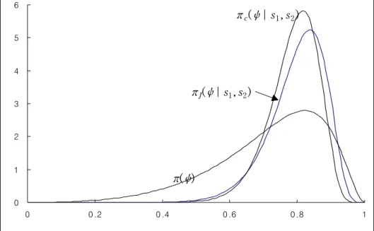
i= 1y_i= 26.234, and the posterior density with respect to noninformative prior

π_J( ψ∣s₁,s₂) = 0.5931ψ⁷(1- ψ)⁶

(1-0.7345ψ)¹⁵ ,0 <ψ < 1. (8) If priors about θ₁ and θ₂ are IG( 3,2) and IG(3,6) then the marginal prior density of ψ is

π( ψ) = 1.1111ψ²(1- ψ)²

(1-0.6667ψ)⁶ ,0<ψ < 1, (9)

(5)

and the posterior density is

π_c( ψ∣s₁,s₂) = 1.4230ψ¹⁰(1- ψ)⁹

(1-0.7219ψ)²¹ ,0 <ψ < 1. (10) Graphs of (8), (9), and (10) are displayed in Figure 1. Table 1 lists Bayes estimates of R obtained from these densities under squared-error loss and LINEX loss. From Table 1, as expected, the Bayes estimates of R decrease as a increase. The estimate obtained with respect to (8) is found to be smaller than the estimates with respect to (9) and (10).

Table 1. Bayes Estimates of R under squared error loss and LINEX loss

a π( ψ) π_c( ψ∣s₁,s₂) π_J( ψ∣s₁,s₂)

-2 -1 0 1 2

0.9550 0.9245 0.8986 0.8734 0.8455

0.8858 0.8762 0.8668 0.8575 0.8482

0.8253 0.8099 0.7964 0.7831 0.7685 (Note: For a = 0, LINEX loss and squared error loss are identical)

(6)

0 1 2 3 4 5 6

0 0.2 0.4 0.6 0.8 1

Figure 1. Prior and Posterior Densities of ψ

Appendix A : Derivation of Jeffreys Prior The likelihood function of (θ1,θ₂) is

l( θ₁,θ₂|S₁,S₂)∝ exp ( - ( S₁/θ₁+ S₂/θ₂))

θ₁ⁿ¹θ₂ⁿ² , θ_i> 0,

from which the likelihood function of ψ = θ2/( θ₁+ θ₂) and ω = θ₁+ θ₂ is given by

l( ψ,ω|S₁,S₂)∝ exp ( - ( S₁/( ( 1 - ψ)ω) + S₂/ψ))

ψ ⁿ²(1- ψ)ⁿ¹ωⁿ . (A.1) The Fisher information matrix for ψ and ω is obtained by taking expectations of the negative of second partial derivatives of the log-likelihood function (A.1).

Observe

l( ψ,ω|S₁,S₂) = constant - n₂logψ - n₁log ( 1 - ψ) - n log ω - 1

ω

(

^(1-ψ)^S¹ ⁺ ^S^ψ²

)

^.

Hence,

I₁₁(ψ, ω) =- E_ψ,ω

{

^∂ψ^∂²² log ( ψ, ω|S₁,S₂)

}

= n₂

ψ² + n₁ (1-ψ)² ,

π_c( ψ∣s₁,s₂)

π_J( ψ∣s₁,s₂)

π( ψ)

(7)

I₁₂(ψ, ω) = 1

ω

(

ⁿ^ψ² ^- ^1-ψⁿ¹

)

^{,and I}²²^{(ψ, ω) =} ωⁿ² . The Fisher information matrix for ψ and ω is then

I( ψ,ω) = ( I_ij)( ψ, ω) = ꀎ

ꀚ

︳︳

ꀏ

ꀛ

︳︳

︳︳ n₂

ψ²+ n₁ (1-ψ)²

1

ω

(

ⁿ^ψ² ^- ^1-ψⁿ¹

)

1

ω

(

ⁿ^ψ² ^- ^1-ψⁿ¹

)

ωⁿ²

, (A.2)

and therefore,

|I( ψ,ω)| = n₁n₂ ψ²(1-ψ)²ω² ,

where |I| denotes the determinant of the matrix I. Hence, the Jeffreys prior for ( ψ, ω) is

π( ψ,ω) ∝ {|I( ψ,ω)| }^1/2

∝ 1

ψ( 1 - ψ)ω , 0 < ψ < 1, ω > 0.

Appendix B : Proof of Theorem 1

The procedure, described in Berger and Bernardo(1989), and Bernardo and Smith(1994, p.326) proceeds as follows:

1. Let π( ω|ψ) be the Jeffreys prior for ω with ψ given, defined by π(ω|ψ)∝( I₂₂(ψ, ω))^1/2. Observe, from (A.2),

I₂₂(ψ, ω) = n ω² . This implies that

π( ω|ψ)∝ 1 ω, ω > 0.

2. Choose an increasing sequence {Λ_i} of subsets of the parameter space Λ for ( ψ, ω), such that ∪

i Λ_i= Λ and π( ω|ψ) has finite mass on Ω_i(ω) = {ω;( ψ, ω)∈Λ_i} for all ψ. Then normalize π_i(ω| ψ) on each Ω_i(ω), obtaining π_i(ω| ψ) = c_i(ψ) ⋅π(ω|ψ)⋅I[ ω∈Ω_i(ω) ], where c_i(ψ) = 1/ ⌠⌡Ωi(ω)π(ω|ψ)dω and I[⋅] is denotes an usual indicator function. Let Λ = ( 0, 1)×( 0, ∞) and Λ_i= ( 0, 1)×( 1/i, i). Let Ω_i(ω) = {ω;1/i < ω < i }, i = 1,2,…, be a suitable sequence of subsets of Λ not depending on ψ, over which π(ω|ψ) can be normalized. It follows that

(8)

c_i(ψ) = 1/ ⌠⌡_1/i1/ωdω = 1 2 log i , and

π_i(ω| ψ) = 1

2ω log i, 1/i < ω < i.

3. Find the marginal reference prior for ψ with respect to π_i( ω|ψ). This is π_i(ψ) ∝ exp

{

^⌠^⌡^Ωⁱ^(ω)^πⁱ(ω|ψ) ⋅ log

[

^I^{|I( ψ,ω)|}²²^{(ψ, ω)}

]

^dω

}

^.

Assuming the integral exists,

π_i(ψ) ∝ exp

{

^⌠^⌡^1/iⁱ ^{2ω log i}¹ ^log

[

^ω²^ψ²^(1-ψ)^ω² ²

]

^1/2^dω

}

= 1

ψ( 1 - ψ) .

4. Define the prior for ( ψ, ω) when ω is a nuisance parameter by π( ψ, ω)∝π( ω |ψ)⋅ lim

i→∞

{

^c^cⁱ^{( ψ}ⁱ^{( ψ)π}⁰^)πⁱⁱ^{( ψ)}^{( ψ}⁰⁾

}

^,

where ψ0 is any fixed point. Assuming the limit exists π( ψ, ω) ∝ 1

ω ⋅ lim

i→∞

{

^{2( log i)ψ}2( log i)ψ( 1 - ψ )⁰^(1-ψ⁰⁾

}

∝ 1

ψ( 1 - ψ)ω , 0 <ψ < 1, ω > 0.

REFERENCES

1. Aitchison, J. and Dunsmore, I.R.(1975). Statistical Prediction Analysis, London: Cambridge University Press.

2. Berger J.O. and Bernardo, J.M.(1989). "Estimating a Product of Means:

Bayesian Analysis with Reference Priors", J. Amer. Stat. Assn, 84, 200-207.

3. Berger J.O. and Bernardo, J.M.(1992). "Ordered Group Reference Priors with Applications to Multinomial Problem", Biometrika, 79, 25-37.

4. Bernardo, J.M.(1979). "Reference Posterior Distribution for Bayesian Inference," J. Royal Stat. Society, B-41, 113-147.

5. Bernardo, J.M. and Smith A.F.M.(1994). Bayesian Theory, NY, John Wiley & Sons.

6. Canfield, R.V.(1970). "A Bayesian Approach to Reliability Estimation Using a Loss Function", IEEE Tr. Rel., 19, 13-16.

7. Dawid, A.P., Stone, N., and Zidek, J.V.(1973). "Marginalization Paradoxes in Bayesian and Structural Inference", J. Royal Stat. Society, B-35,

(9)

189-233.

8. Enis, P. and Geisser, S.(1971). "Estimation of Probability that Y <X" , J.

Amer. Stat. Assn, 66,162-168.24.

9. Ferguson, T.S.(1967), Mathematical Statistics: A Decision Theoretic Approach, NY: Academic Press.

10. Feynman, R.P.(1987). "Mr. Feynman goes to Washington", Engineering and Science, California Institute of Technology", CA, 6-22.

11. Gupta, R.D. and Gupta, R.C.(1988). "Estimation of

P( Y_p> Max( Y₁,Y₂,…,Y_{p - 1})) in the Exponential Case", Comm.

Stat-Theory & Methods, 17, 911-924

12. Varian, H.R.(1975). "A Bayesian Approach to Real Estate Assessment.

S.E.Feinberg and A. Zellner, Eds.", Studies in Bayesian Econometrics and Statistics in Honor of L.J.Savage, NY:North-Holland, Pub.

Co.,195-208.

13. Zellner, A.(1986). "Bayesian Estimation and Prediction Using Asymmetric loss Function", J. Amer. Stat. Assn., 81,446-451.

14. Zellner, A. and Geisel, M.S.(1968). "Sensitivity of Control to Uncertainty and Form of the Criterion Function", in the Future of Statistics, ed.

Donald, G. W. NY, Academic Press, 269-289.

[ received date : Apr. 2003, accepted date : Jul. 2003 ]