Article https://doi.org/10.14478/ace.2019.1040
1. Introduction1)
Flow coating processes involving mono-dispersed colloidal particles have recently attracted considerable interest for a number of industrial applications, such as chemical sensors, displays, and conductive films.
The most commonly used coating techniques in common are that blade coating, knife coating, and doctor blade coating (DBC), in which a functional coating progresses continuously to pattern colloidal mono-lay- ers or ordered structures on a substrate.
In the DBC process, a fixed blade generates a shear force on the upper part of a mixed slurry with a moving substrate, and creates a flat slurry through the gap between the processed slurry and the blade.
The shear force applied by the blade induces an interesting phenomen- on in the slurry containing the mono-dispersed colloidal particles (also called a suspension): the Newtonian fluid with suspended particles ex- hibits non-Newtonian behavior. Such processes have also dealt with a variety of particle dispersions with complex rheology in which a large concentration of particles is generated, referred to as shear thickening
† Corresponding Author: Kyushu University,
Department of Chemical Engineering, Faculty of Engineering, Nishi-ku, Fukuoka 819-0395, Japan
Tel: +81-92-802-2774 e-mail: g.kim@kyudai.jp
pISSN: 1225-0112eISSN: 2288-4505 @ 2019 The Korean Society of Industrial and Engineering Chemistry. All rights reserved.
(ST)[1-4]. In some cases, the immersed particle energy distribution rate induced by the shear deceases with increasing shear rate, which is re- ferred to as shear thinning. Meanwhile, the energy dissipation rate in- duced by the shear stress increases with increasing shear rate, resulting in ST. Although the cases resulting in ST are less common than the cases of shear thinning, the cases of ST have been researched ex- tensively in the fields of colloidal and non-colloidal suspensions, with many published papers. ST behavior can directly affect the coating process[5]. The stresses resulting from the concentrated particles need to be accurately predicted, as the overloading of stresses in a material can cause serious damage and failure. Kim et al. found that ST fluids tend to accumulate and exhibit a nonlinear steady-state profile, causing the film coating thickness to become uneven[6]. In a study of the rela- tionship between the coating speed and the effect of ST, it was found that ST can limit the coating speed through non-Newtonian behav- ior[7]. Furthermore, ST can damage coating transport process devices, mixing blades, and motors through overloading caused by concentrated dispersions[2], leading to a poor coating quality[8]. As such, in many industrial application fields utilizing coating processes, these un- desirable phenomena have resulted in various attempts to adopt ST flu- ids for applications while controlling their properties to minimize harmful effects. In these efforts, many questions have arisen regarding the suspension mechanism with consideration of ST. However, although
전단 흐름을 갖는 서스펜션 내부 나노 입자의 유변학적 특성 연구
김 구†⋅후카이 준⋅히로나카 슈지
규슈대학교 화학공학과
(2019년 5월 24일 접수, 2019년 6월 17일 심사, 2019년 6월 27일 채택)
Rheological Modeling of Nanoparticles in a Suspension with Shear Flow
Gu Kim†, Jun Fukai, and Shuji Hironaka
Department of Chemical Engineering, Faculty of Engineering, Kyushu University, Nishi-ku, Fukuoka 819-0395, Japan (Received May 24, 2019; Revised June 17, 2019; Accepted June 27, 2019)
Abstract
Shear thickening is an intriguing phenomenon in the fields of chemical engineering and rheology because it originates from complex situations with experimental and numerical measurements. This paper presents results from the numerical modeling of the particle-fluid dynamics of a two-dimensional mixture of colloidal particles immersed in a fluid. Our results reveal the characteristic particle behavior with an application of a shear force to the upper part of the fluid domain. By combining the lattice Boltzmann and discrete element methods with the calculation of the lubrication forces when particles approach or re- cede from each other, this study aims to reveal the behavior of the suspension, specifically shear thickening. The results show that the calculated suspension viscosity is in good agreement with the experimental results. Results describing the particle deviation, diffusivity, concentration, and contact numbers are also demonstrated.
Keywords: Nano-particles, Thin film, Suspension, Shear thickening, Non-Newtonian fluid
many researchers have studied ST fluids that act reversibly as smart fluids, their complex behavior has not yet been elucidated. The first at- tempt to reveal their details was the micro-structure experiments con- ducted by Hoffman[9]. He noted that a number of polymer particle suspensions under shear exhibited ordered, hexagonally packed layers before the ST transition. Hoffman also proposed that at a low shear rate, these layers resulted in a shear thinning region, but they resulted in ST at high shear rates[10]. Although common rheology measure- ments have made it possible to find particle clusters formed by ST ex- perimentally, the details of the microscopic particle dynamics and their mutual interactions are still ambiguous. To provide explanations, nu- merical simulations have become an important tool, with increasing computational techniques to meet the demands for precise predictions of the particle motion in a fluid. Many investigations using mathemat- ical approaches have attempted to achieve a deeper understanding be- yond that available through experimental studies owing to measurement limitations. Yang et al. investigated the effect of hydrodynamic par- ticle-fluid interactions in the flow, vorticity, and gradient directions with varying shear rates[11]. Xin et al. studied the relationship be- tween the strength of the hydrodynamic ST and the distribution of the hydrodynamic clusters, and found that the network of clusters formed a jamming structure at high shear rate and increasing viscosity[12].
Chen et al. noted that the string curve formed by the particle structure rotates with other particles under compression[13]. However, quantita- tive predictions, such as the onset of ST and details of the particle mo- tion tendency under ST, are still lacking. A breakthrough for solving both the particle-fluid and particle-particle interactions in a suspension has been provided by particle-based simulation methods, which have shown good agreement for simulating the fluid flow with solids at both microscopic and macroscopic scales. For instance, Stokesian dynamics (SD) has often been used. This method provides a description of the interaction of particles in a multiphase flow. Many studies have applied SD to determine the effect of the suspension viscosity and volume fraction, ϕ, and the results have been compared with experimental results. However, this method provides only non-dynamic particle behavior. For solid mechanics, the discrete elements method (DEM), which has been widely adopted for problems relating to granular mate- rial dynamics, is selected for this study. In addition, the coupling of DEM with the lattice Boltzmann method (LBM) has been used to in- troduce the interactions between the fluid and particles. Furthermore, in this study, the lubrication forces to overcome their divergent behav- iors are also considered, because the ST behavior arises from the grouping of particles through hydrodynamic lubrication forces, which should be considered when determining the microscopic origins of the non-Newtonian flow behavior. Thus, this study contributes novel re- sults in several aspects. First, we investigated and calculated the lu- brication forces with a coupled Eulerian/Lagrangian method. Second, we clearly demonstrated the onset of shear thickening, which can pro- vide valuable guidance for future development of suspension models.
Finally, this study also allows to determine the suspension viscosity in a dynamic simulation using the force balance model.
This paper presents a mathematical approach that will be valuable
Figure 1. Discretization of the position and velocity space for a D2Q9 lattice.
for understanding ST behavior. The remainder of the paper is organized as follows: Section 2 describes the methodology of the LBM and DEM, including the lubrication force model; Section 3 gives the numerical re- sults, including the deviation, diffusivity, concentration, and contact number; and finally, some conclusions are presented in Section 4.
2. Model Description
2.1. LBM
LBM is a representative method to approach the Navier-Stokes sol- ution and a mesoscale discrete velocity model for solving problems of fluid flow[4]. LBM has several advantages such as using a regular grid with no need for rearrangement of the equation during the calculation process[14], unlike the conventional finite element method (FEM) and finite volume method (FVM). It utilizes the coordinated discretization of the physical velocity, physical spaces, and time, tracking the evolu- tion of a vector defined by the expected density distribution, f. This evolution consists of two parts: the streaming part and the collision part. The density distribution functions are calculated using the lattice Boltzmann equation (LBE) with the Bhatnagar-Gross-Krook (BGK) op- erator[15], and is defined as follows:
=
(1)
= (2)
In Eq. (1), the right side represents the collision part, the left side is the streaming part, x is the spacing, t is the time, is the velocity direction, and is the dimensionless relaxation time related to the fluid viscosity (in this study, ≈ 0.6).
The equilibrium distribution function, , in Eq. (2) is defined as:
=
(3)In Eq. (3), the is the initial velocity of fluid, the weighting factor,
, is 4/9 for = 0; 1/9 for = 1, 2, 3, and 4; and 1/36 for =
447
5, 6, and 7. Figure 1 illustrates the momentum discretization for a two-dimensional calculation, where the virtual fluid particles at each node move to eight intermediate neighbors with eight corresponding velocity vectors: = , = , = , = ,
= , = , = , and = , where is equal to . The different velocity sets are used for different purposes. These velocity sets by DdQq, where d is the num- ber of dimensions the velocity and is the set’s number of velocities.
In this study D2Q9 was used.
Furthermore, Eq. (1) is solved in two steps as follows:
⋅Collision step:
= (4a)
⋅Streanubg step:
= (4b)
where is the post-collision density distribution. For efficient calcula- tion, the post-collision state obtained by splitting the computational pro- cedure can reduce the steps to store both and , and is appropriate in one time for a dynamic flow calculation.
The representative single relaxation time (SRT) BGK collision oper- ator depends on a single relaxation time, . However, such an SRT BGK model for the collision has the fundamental drawback of a solution in- accuracy in which it is difficult to eliminate the acoustic mode at high Reynolds numbers. To overcome this serious problem, in this calcu- lation, a multi-relaxation time (MRT)[16] collision operator is applied.
A detailed discussion of the MRT calculation conditions are described in Refs.[4,17].
The macroscopic values are defined by following equations:
= (5)
= (6)
where is 9 in D2Q9 for the two-dimensional calculation.
2.2. DEM
A widely utilized approach for the calculation of the solid phase is DEM, originally derived from molecular dynamics and modeled by Cundall[18], in which the explicit temporal integration of the mo- mentum balance is calculated for the particle kinematics.
The behavior of each particle in DEM is determined as a discrete element. The governing equation for the particle motion of each ele- ment is based on Newton’s second law including the following values:
particles with mass , position , velocity , angular velocity , and acceleration ; is the inertia of particle .
= (7)
= (8)
The calculation of the external forces acting on each particle, , in the same simulation time includes the contact working force, , the hydrodynamic force, , and the lubrication force, ; , , and
are the torques due to the contact, hydrodynamic, and lubrication forces, respectively. In particular, includes two components: the normal force, , and the tangential force, , between two overlapping particles, and , as follows:
= (9)
where and are the unit vectors in the normal and tangential direc- tions, respectively. The detailed mechanism of the DEM calculation can be found in Refs.[19-23].
2.3. Coupled LBM and DEM
To solve the particle movement on the lattice grid with the fluid si- multaneously[24], with the previously proposed methods[25-28], in this calculation, the interpolated bounce-back (IBB) scheme proposed by Bouzidi et al.[28] was selected to apply a non-slip boundary condition between the fluid nodes and the particles. This condition can be im- posed along the particle surface for the fluid-solid interaction. Owen et al. introduced a revised LBM where overlapping particles in the lat- tice grid can be solved using an immersed moving boundary con- dition[29]. In the IBB scheme, the hydrodynamic forces acting on the particles are obtained using the momentum exchange method[13]. The average force on the boundary links, , imposed by the fluid and solid boundary nodes is calculated as follows:
=
̂ ̂ (10)
where ̂ is in the opposite direction of and is the inverse direction of .
The total hydrodynamic force is calculated by the sum of :
=
(11)
Additionally, the process for determining the total hydrodynamic tor- que is given by the following:
= × (12)
= (13)
where =
.
2.4. Efficient contact detection algorithm
As an efficient calculation method for a large number of particles, the Verlet list algorithm was selected as an efficient contact detection algorithm[30]. This algorithm can detect each particle when it approaches contact with a neighboring particle by whether it is in the calculation list based on the cut-off radius[31].
2.5. Calculation of lubrication forces
The lubrication forces when a particle approaches a neighboring par- ticles are considerable. These forces tend to arise from changes in the distance between particle surfaces when approaching or receding, i.e., squeezing or sucking in fluid.
Honig et al. proposed a concept for the computation of lubrication forces[32]. Despite the need for lubrication forces to act in the tangen- tial direction and the torque calculation, the approach proposed by Honig involves only the normal force. Thus, it is necessary to perform a more complete calculation including the tangential components. Dance et al. recently proposed lubrication forces with the tangential compo- nents and torques for particle-particle and particle-wall interactions[33].
The mechanism was derived using an asymptotic expansion for two particles or a particle that is near the wall, as given by Eqs. (14) and (15), respectively:
= ⋅
(14a)
=
(14b)
=
× × (14c)
where is the normal force; is the sliding force; is the sliding torque; the relative velocity is defined as = ; is the unit nor- mal vector; the sliding velocity, , is equal to ⋅; the slid- ing velocity considering the rotational motion is = , with
= × and = ×, where the vector pointing from the center of each particle to its surface is = and = ; and the relative distance, , is
, where the separation distance, , is equal to
.
Additionally, as noted above, the interaction between the wall and particles is required for the lubrication forces; the normal force, , sliding force, , and sliding torque, , are given by the following:
= ⋅
(15a)
=
(15b)
=
× × (15c)
where , , and are calculated using same method as in the par- ticle-particle interaction in Eqs. (14a)~(14c).
An important problem is the divergent behavior when is 0. The problem is to solve for an accurate numerical simulation while avoid- ing unrealistic results. Some accepted approaches to overcome di- vergent behavior such as that of the lubrication forces have been sug- gested[34], implemented as the following form:
=
(16)
In Eq. (16), is the slip length, and the right sides of Eqs. (14)~(15) are multiplied by if . If , and =
are used to reduce the magnitude of the lubrication forces. In this study, the value of was set as 0.1.
2.6. Viscosity evaluation
The estimation model for the viscosity is derived from Newton’s law of viscosity as follows:
= γ́ (17)
where is the shear stress, which can also be defined as:
=
(18)
where is the length of part inducing the shear force and is the shear force applied to the upper domain.
The force balance for the forces considered in this study is given by the following:
= 0 (19)
where is the sum of the lubrication forces from the particles and
is the hydrodynamic stress from the fluid, which is given by the following:
= (20)
can be obtained from the local velocity gradient as follows:
=
(21)
449
where is the x-directional fluid velocity and is the height of the computational fluid domain. The velocity sampling position ( = ) is near the upper wall generating the shear force, because the calculation domain has a shorter height than width. Thus, the sampling position is sufficiently affected by the shear. The viscosity, , is defined as:
=
γ́
(22)
The starting point for is calculated as the sum of for all par- ticles due to the shorter height of the domain as follows:
= (23)
Similar to , is obtained with the following:
=
γ́
(24)
Finally, is the sum of and .
3. Results and Discussion
The fluid domain size is 620 r × 36 r (width × height), where is the radius of a particle. Particles were randomly placed on the lattice grid in locations where there was no contact with any of the surround- ing walls or neighboring particles. For the moving boundary condition on the upper wall for the shear flow, the half-way bounce-back method was applied[36,37], and thus this method was also used for the no-slip boundary condition. The fluid distribution when contacting the wall boundary condition is bounced back in the opposite direction, and then the microscopic boundary rule creates the no-slip condition as follows:
= ̂
(25)
where ̂ is the fluid distribution after collision and is the velocity along the wall.
The details of the parameters used in these simulations are listed in Table 1. It is worth noting that in this study, the Brownian motion was neglected owing to the high Peclet number resulting from the large ap- plied shear rates.
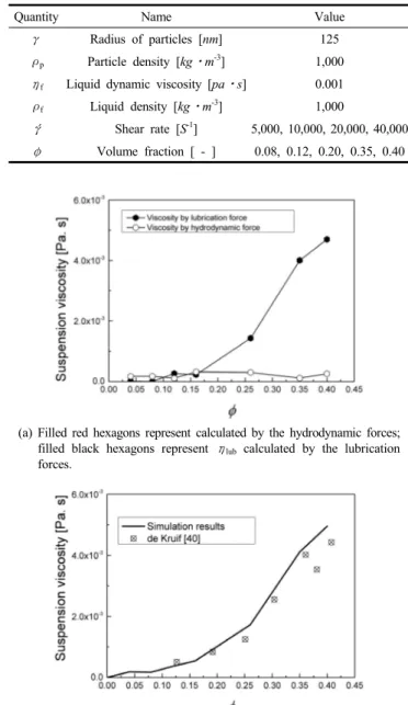
3.1. Evaluation of the viscosity calculation
The viscosity was calculated with the hydrodynamic forces, , and the lubrication forces, , using Eqs. (22) and (24), respectively. As illustrated in Figure 2 (a), increases exponentially, i.e., it exhibits a characteristic power-law behavior ( ≈ , with ≈ 2) due to the contribution of the particle interactions. Meanwhile, even with increas- ing , is somewhat enhanced because of the reduced distances of
Quantity Name Value
γ Radius of particles [nm] 125
ρp Particle density [kg⋅m-3] 1,000 ηf Liquid dynamic viscosity [pa⋅s] 0.001 ρf Liquid density [kg⋅m-3] 1,000
γˊ Shear rate [S-1] 5,000, 10,000, 20,000, 40,000 ϕ Volume fraction [ - ] 0.08, 0.12, 0.20, 0.35, 0.40 Table 1. Parameters Used in the Simulation
(a) Filled red hexagons represent calculated by the hydrodynamic forces;
filled black hexagons represent ηlub calculated by the lubrication forces.
(b) Numerical calculation of the viscosity compared to the experimental results of de Kruif et al.[35] at γˊ = 40,000 s-1.
Figure 2. Viscosity calculation results.
the particle displacement[38]. As a general explanation pertaining to these results, the hydrodynamic contribution remains stable, but the contact forces generate force networks that can obey the thickening parts where the hydrodynamic interaction is insufficient[39]. Figure 2 (b) illustrates the numerical results for with changing , compared to experimental results mono-dispersed nanoparticles in a suspen- sion[35]. The results show that increases sharply from ≈ 0.3, which is in good agreement with the experimental results. According to a well-known mechanism[40], dilation, this large increase in is caused by the dilation of the particle packing with the onset of ST. Furthermore, such dilation would require that the shear stress overcome the particle stresses preventing compressive shear between particles.
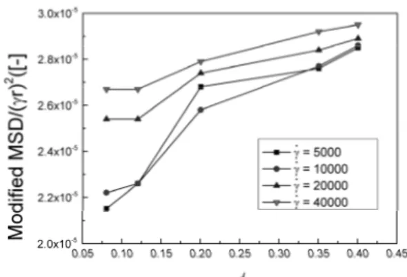
Figure 3. Modified mean squared displacement.
3.2. Average squared displacements
To elucidate the particle displacement mechanism, Figure 3 illustrates the results for the modified mean squared displacement (MSD)[41] fre- quently used in statistical mechanics as well as in biophysics and envi- ronmental engineering[42]. The modified MSD can be used to estimate the deviation of the position of particles from the average particle positions. In other words, the ASD the pattern of how particles are dis- persed in fluid, the modified MSD is given by the following:
〈〉 = 〈 〉 (26)
where is the center coordinate of the particles. The results were ave- raged over all times based on the number of particle results for each case.
It is noteworthy that in this study, dilute conditions, notably ≤ 0.03, were not considered, as the interaction between the particles was not significant[43].
With increasing , it is observed that the modified MSD increases in all cases. With γ́ = 5,000 and 10,000 s-1, the modified MSD are smaller than for the other cases, which indicates that the particle spreading patterns are similar and have not deviated. Above = 0.3, the modified MSD in all cases are similar because an increasing num- ber of particles are affected by the shear. In addition, such particles are formed in which the repulsive forces between particles cannot be over- come by the short-range hydrodynamic . The other cases indicate more deviated particles, and stable results (modified MSD ∝) are ob- tained even with the increase in .
3.3. Diffusivity
Figure 4 illustrates the results for the particle diffusivity, which was quantified using the velocity autocorrelation function in the y-direction,
= 〈〉, as follows:
= (27)
As can be seen in Figure 4, increases with increasing γ́. Except for γ́ = 40,000 s-1, the other results all exhibit a plateau characteristic.
Figure 4. Diffusivity according to Eq. (27).
In particular, for = 0.40 and γ́ = 40,000 s-1 exhibits a decrease. This reduced can be regarded as the onset of ST from = 0.35. ST gen- erally does not occur in a dilute suspension, but its characteristics are typically observed around 0.30 < < 0.40 as intermediate packing fractions[44,45]. Considering an understanding of how ST occurs rheo- logically, several reviews suggest that a predominantly accepted mech- anism is the hydro-cluster mechanism[46]. In this mechanism, the im- mersed particles under shear may push more closely into each other through the arising of lubrication hydrodynamic forces[47]. Furthermore, such particles then stick together to form clusters above a critical shear rate. If the accumulated particles are dispersed, the viscous drag forces between the lubrication gaps for each particle must be overcome. The cluster magnitude increases with increasing γ́[48], which results in the increase in viscosity, and thus hydro-clustering is a trigger for the on- set of ST[49].
3.4. Concentration coefficient
To estimate the heterogeneous state from the particle formation, whether concentrated or not, the concentration coefficient, , averaged by the time and number of particle results is used as the relative mean difference. The mean of the difference between every possible pair of particles is evaluated by the summary statistical measurement of the in- equality in the particle distribution. Furthermore, if is decreased, more particles may be close together or grouped. The concentration co- efficient is given by the following equation:
= 〈 〉 (28)
where is the mean distance between particles and and are the number of particles. Overall, is decreased with increasing in all cases, as illustrated in Figure 5. The for γ́ = 20,000, 10,000, and 5,000 s-1 are similar. However, interestingly, the results for with γ́
= 40,000 s-1 are lower than in the other cases, which indicates that chains of hydro-clusters composed of concentrated particles are parti- ally formed as the number of grouped particles increases, despite the higher diffusivity illustrated in Figure 4. It can be explained that hy- dro-clusters could be formed in this regime through the prominent con-
451
Figure 5. Concentration coefficient results.
Figure 6. Physical particle contact numbers at γˊ = 40,000 s-1.
gestion effect[50], and the formation of such aggregates can be a jam flow[51].
3.5. Contact analysis
To support the previous explanations of the observed particle behav- ior at γ́ = 40,000 s-1, the physical particle contact number, , divided by the number of particles and also averaged over all times, for the interaction of each neighboring particle is illustrated in Figure 6. This contact analysis is crucial for a suspension study because Hoffman et al.[9] suggested that the physical contacts between particles causes the ST phenomenon from ordered to disordered particle formations. With the same trend as previously observed for at γ́ = 40,000 s-1 in Figure 4, tends to increase to = 0.35, and decrease slightly at
= 0.40. In other words, the trend in is related to the particle diffu- sivity. Notably, the contact of particles with each neighboring particle results in the formation of contact networks that can be extended.
4. Conclusions
In conclusion, nanoparticles in a suspension were examined in this study using the combined DEM-LBM model with added calculation of the lubrication forces and the shear flow. The results provide a deep comprehension of ST with details of the positioning and concentration of particles with varying diffusivity.
⋅The lubrication forces contribute predominantly to increase the vi-
scosity of a suspension, while the viscosity was slightly increased by hydrodynamic forces, presenting a good agreement with the experimental data.
⋅The difference in the deviation of particles as a function of at higher γ́ is constant because the short-range hydrodynamic lu- brication forces can be dominate.
⋅The particle diffusivity reveals that the onset of ST is at = 0.35 as intermediate packing fractions.
⋅At γ́ = 40,000 s-1, concentrated particles chains composed of hy- dro-clusters are partially formed. This concentrated particles would be jam flow.
⋅The ST is strongly related to the particle contact and particle ve- locity trends, and the contact networks of particles can be extended when higher γ́.
This investigation provides a further illustration of the complex na- ture of ST behavior.
References
1. M. Schmitt, M. Baunach, L. Wengeler, K. Peters, P. Junges, P.
Scharfer, and W. Schabel, Slot-die processing of lithium-ion bat- tery electrodes-coating window characterization, Chem. Eng. Pro- cess., 68, 32-37 (2013).
2. H. A. Barnes, Shear-thickening (“Dilatancy”) in suspensions of non aggregating solid particles dispersed in newtonian liquids, J. Rheol., 33, 329-366 (1989).
3. S. Khandavalli and J. Rothstein, Extensional rheology of shear-thicken- ing nanoparticle dispersions in an aqueous polyethylene oxide sol- utions, J. Rheol., 58(2), 411-431 (2014).
4. H. Liu, Q. Kang, C. R. Leonardi, S. Schmieschek, A. Narváez, B.
D. Jones, J. R. Williams, A. J. Valocchi, and J. Harting, Multiphase lattice Boltzmann simulations for porous media applications, Comput.
Geosci., 20(4), 777-805 (2016).
5. S. Khandavalli, J. A. Lee, M. Pasquali, and J. P. Rothstein, The effect of shear-thickening on liquid transfer from an idealized gra- vure cell, J. Nonnewton. Fluid Mech., 221, 55-65 (2015).
6. K. T. Kim and R. E. Khayat, Transient coating flow of a thin non-Newtonian fluid film, Phys. Fluids, 14, 2202-2215 (2002).
7. T. Tsuda, Coating flows of power-law non-newtonian fluid in slot coating, J. Soc. Rheol. Jpn., 38(4-5), 223-230 (2010).
8. K. M. Beazley, Industrial aqueous suspensions, in: K. Walters (ed.), Rheometry: Industrial Applications, 339-413, Research Studies Press, Chichester UK (1980).
9. R. L. Hoffman, Explanations for the cause of shear thickening in concentrated colloidal suspensions, J. Rheol., 42, 111-123 (1998).
10. R. L. Hoffman, Discontinuous and dilatant viscosity behavior in concentrated suspensions: III. Necessary conditions for their occur- rence in viscometric flows, Adv. Colloid Interface Sci., 17(1), 161-184 (1982).
11. M. Yang and E. S. G. Shaqfeh, Mechanism of shear thickening in suspensions of rigid spheres in Boger fluids. Part II: Suspensions at finite concentration, J. Nonnewton. Fluid Mech., 234, 51-68 (2016).
12. X. Bian, S. Litvinov, M. Ellero, and N. J. Wagner, Hydrodynamic shear thickening of particulate suspension under confinement, J.
Nonnewton. Fluid Mech., 213, 39-49 (2014).
13. Y. Chen, Q. Cai, Z. Xia, M. Wang, and S. Chen, Momentum-ex- change method in lattice Boltzmann simulations of particle-fluid interactions, Phys. Rev. E, 88(1), 013303-1-15 (2013).
14. M. C. Sukop and D. T. Thorne, Lattice Boltzmann Modeling: An Introduction for Geoscientists and Engineers, 31-35, Springer (2007).
15. G. V. Krivovichev, Linear Bhatnagar-Gross-Krook equations for simulation of linear diffusion equation by lattice Boltzmann meth- od, Appl. Math. Comput., 325, 102-119 (2018).
16. L. S. Lin, H. W. Chang, and C. A. Lin, Multi relaxation time lat- tice Boltzmann simulations of transition in deep 2D lid driven cav- ity using GPU, Comput. Fluids, 80(10), 381-387 (2013).
17. K. Chen, Y. Wang, S. Xuan, and X. Gong, A hybrid molecular dynamics study on the non-Newtonian rheological behaviors of shear thickening fluid, J. Colloid Interface Sci., 497(1), 378-384 (2017).
18. P. A. Cundall and O. D. L. Strack, A discrete numerical model for granular assemblies, Geotechnique, 29(1), 47-65 (1979).
19. M. Kuanmin, Y. W. Michael, X. Zhiwei, and C. Tianning, DEM simulation of particle damping, Powder Technol., 142(2), 154-165 (2004).
20. W. Smith, D. Melanz, C. Senatore, K. Iagnemma, and H. Peng, Comparison of discrete element method and traditional modeling methods for steady-state wheel-terrain interaction of small vehicles, J. Terramechanic, 56, 61-75 (2014).
21. S. Laryea, M. S. Baghsorkhi, J. F. Ferellec, G. R. McDowell, and C. Chen, Comparison of performance of concrete and steel sleepers using experimental and discrete element methods, Transp. Geotech., 1(4), 225-240 (2014).
22. P. P. Procházka, Application of discrete element methods to frac- ture mechanics of rock bursts, Eng. Fract. Mech., 71(4), 601-618 (2004).
23. H. P. Zhu and A. B. Yu, A theoretical analysis of the force models in discrete element method, Powder Technol., 161(2), 122-129 (2006).
24. I. Klaus, T. Nils, and R. Ulrich, Simulation of moving particles in 3D with the Lattice Boltzmann method, Comput. Math. Appl., 55, 1461-1468 (2008).
25. O. Filippova and D. Hänel, Grid refinement for lattice-BGK mod- els, J. Comput. Phys., 147, 219-228 (1998).
26. R. Mei, L. S. Luo, and W. Shyy, An accurate curved boundary treatment in the lattice Boltzmann method, J. Comput. Phys., 155, 307-330 (1999).
27. C. Chang, C. H. Liu, and C. A. Li, Boundary conditions for lattice Boltzmann simulations with complex geometry flows, Comput. Math.
Appl., 58(5), 940-949 (2002).
28. M. Bouzidi, M. Firdaouss, and P. Lallemand, Momentum transfer of a boltzmann-lattice fluid with boundaries, Phys. Fluids, 13, 3452-3459 (2001).
29. D. R. J. Owen, C. R. Leonardi, and Y. T. Feng, An efficient frame- work for fluid-structure interaction using the lattice Boltzmann meth- od and immersed moving boundaries, Int. J. Numer. Methods Eng., 87(1), 66-95 (2011).
30. L. Verlet, Computer “Experiments” on classical fluids. I. Thermody- namical properties of Lennard-Jones molecules, Phys. Rev., 159(1), 98-103 (1967).
31. H. Grubmuller, H. Heller, A. Windemuth, and K. Schulten, Generalized verlet algorithm for efficient molecular dynamics sim- ulations with long-range interactions, Mol. Simul., 6, 121-142 (1991).
32. E. P. Honig, G. J. Roeberse, and P. H. Wiersema, Effect of hydro- dynamic interaction on coagulation rate of hydrophobic colloids, J.
Colloid Interface Sci., 36, 36-97 (1971).
33. S. L. Dance and M. R. Maxey, Incorporation of lubrication effects into the force-coupling method for particulate two-phase flow, J.
Comput. Phys., 189, 212-238 (2003).
34. O. I. Vinogradova, Drainage of a thin liquid-film confined between hydrophobic surfaces, Langmuir, 11, 2213-2220 (1995).
35. C. G. de Kruif, E. M. F. van Iersel, A. Vrij, and W. B. Russel, Hardsphere colloidal dispersions - Viscosity as a function of shear rate and volume fraction, J. Chem. Phys., 83, 4717-4725 (1985).
36. T. Zhang, B. Shi, Z. Guo, Z. Chai, and J. Lu, General bounce-back scheme for concentration boundary condition in the lattice-Boltzmann method, Phys. Rev., 85, 016701-1-14 (2012).
37. Y. Zong, C. Peng, Z. Guoc, and L. P. Wang, Designing correct fluid hydrodynamics on a rectangular grid using MRT lattice Boltzmann approach, Comput. Math. Appl., 72, 288-310 (2016).
38. B. J. Maranzano and N. J. Wagner, The effects of interparticle in- teractions and particle size on reversible shear thickening: Hard-sphere colloidal dispersions, J. Rheol., 45, 1205-1222 (2001).
39. I. R. Peters, S. Majumdar, and H. M. Jaeger, Direct observation of dynamic shear jamming in dense suspensions, Nature, 532, 214-217 (2016).
40. E. Brown and H. M. Jaeger, The role of dilation and confining stresses in shear thickening of dense suspensions, J. Rheol., 56(4), 875-923 (2012).
41. A. Sierou and J. F. Brady, Shear-induced self-diffusion in non-col- loidal suspensions, J. Fluid Mech., 506, 285-314 (2004).
42. N. Tarantino, J. Y. Tinevez, E. F. Crowell, B. Boisson, R. Henriques, M. Mhlanga, F. Agou, A. Israël, and E. Laplantine, TNF and IL-1 exhibit distinct ubiquitin requirements for inducing NEMO-IKK supramolecular structures, J. Cell Biol., 204(2), 231-245 (2014).
43. A. Einstein, Eine neue bestimmung der molekldimensionen, Ann.
Phys. (Berl.), 324(2), 289-306 (1906).
44. E. Nazockdast and J. F. Morris, Microstructural theory and the rheology of concentrated colloidal suspensions, J. Fluid Mech., 713, 420-452 (2012).
45. N. J. Wagner and J. F. Brady, Shear thickening in colloidal dis- persions, Phys. Today, 62, 27-32 (2009).
46. J. Bergenholtz, J. F. Brady, and M. Vicic, The non-Newtonian rheology of dilute colloidal suspensions, J. Fluid Mech., 456, 239-275 (2002).
47. N. J. Wagner and J. F. Brady, Shear thickening in colloidal dis- persions, Phys. Today, 62(10), 27-32 (2009).
48. R. G. Egres, F. Nettesheim, and N. J. Wagner, Rheo-SANS inves- tigation of acicular-precipitated calcium carbonate colloidal suspen- sions through the shear thickening transition, J. Rheol., 50(5), 685-709 (2006).
49. H. M. Jaeger, S. R. Nagel, and R. P. Behringer, Granular solids, liquids, and gases, Rev. Mod. Phys., 68(4), 1259-1273 (1996).
50. W. Huang, Y. Wu, L. Qiu, C. Dong, J. Ding, and D. Li, Tuning rheological performance of silica concentrated shear thickening flu- id by using graphene oxide, Adv. Condens. Matter Phys., 2015, 734250 (2015).
51. N. J. Wagner, E. D. Wetzel, G. Ronald, and J. R. Egres, Shear thickening fluid containment in polymer composites, US Patent 0234572 (2006).