Printed in the Republic of Korea
http://dx.doi.org/10.5012/jkcs.2013.57.3.370
Correlation of Liquid-Liquid Equilibrium of Four Binary Hydrocarbon-Water Systems, Using an Improved Artificial Neural Network Model
Hui-Chao Lv* and Yan-Hong Shen
College of Chemical & Environmental Engineering, Anyang Institute of Technology, Anyang 455000, China.
*E-mail: [email protected]
(Received December 24, 2012; Accepted April 30, 2013)
ABSTRACT. A back propagation artificial neural network model with one hidden layer is established to correlate the liquid- liquid equilibrium data of hydrocarbon-water systems. The model has four inputs and two outputs. The network is systemati- cally trained with 48 data points in the range of 283.15 to 405.37K. Statistical analyses show that the optimised neural net- work model can yield excellent agreement with experimental data(the average absolute deviations equal to 0.037% and 0.0012% for the correlated mole fractions of hydrocarbon in two coexisting liquid phases respectively). The comparison in terms of average absolute deviation between the correlated mole fractions for each binary system and literature results indicates that the artificial neural network model gives far better results. This study also shows that artificial neural network model could be developed for the phase equilibria for a family of hydrocarbon-water binaries.
Key words: Hydrocarbon-water system, Liquid-liquid equilibrium, Artificial neural network, Correlation
INTRODUCTION
Since water is present in natural gas and petroleum reser- voirs, the research on the behavior of water in hydrocar- bon systems is significant for a large number of chemical engineering applications such as the exploitation of reservoirs, refining, the guarantee of product quality and environmental protection, etc.1 In addition to reducing the number of experimental data points to be measured, accurate com- putational models and correlation methods for the phase equilibria of hydrocarbon-water systems can be used to predict the maximum water content of fuels and to assist in the design of separation equipment.1,2
In the field of thermodynamics, the statistical theoretical models such as MPHC (Modified Perturbed Hard Chain), SAFT (Statistical Associating Fluid Theory) and CPA (Cubic Plus Association)5 are often employed to simulate phase equilibria in petroleum industry. Wang et al. cor- related the liquid-liquid equilibrium data of four binary hydrocarbon-water systems by means of MPHC.3 SAFT was used to model liquid-liquid and liquid-vapor equilibrium of binary systems containing water with methane, ethane, CO2 or H2S by Huynh et al.1 Riaz et al. studied the distribution of monoethylene glycol and methanol in hydrocarbon- water systems using CPA.4 Besides, some simple models based on cubic EoS (Equation of State) or activity coefficient equation still represent a great interest for industrial appli- cations. Panagiotopoulos et al. proposed SRKm (Soave-
Redlich-Kwong modified) EoS and modeled reservoir flu- ids in the presence of associating compounds.5 Wang et al.
correlated the liquid-liquid equilibrium data of four binary hydrocarbon-water systems using NRTL (Non Random Two Liquid) activity coefficient model.3 NRTL-PR (Peng- Robinson) EoS was applied to modeling of nonideal sys- tems by Neau et al.6 and new interaction parameters are proposed for a wide variety of mixtures composed of very asymmetric compounds by Escandell et al.7 Gebreyohannes et al. used the QSPR (Quantitative Structure-Property Relationship) methodology to generalize the interaction parameters of the NRTL model for many binary systems.8 Although these models contribute much to the research on the fluid phase equilibria, all without exception involve a certain amount of empiricism to determine mixture con- stants, through fitting experimental data and using vari- ous arbitrary mixing rules, making it difficult to select the appropriate model for a particular case. Hence, it is an arduous task for a non expert in thermodynamics to deal with phase equilibria using these models.
On the other hand, artificial neural network (ANN), which can be viewed as a powerful and efficient computational tool with an inherent ability to extract from experimental data the highly non linear and complex relationships between the variables of the problem handled, has gained exten- sive attention in the field of data processing.9 As far as phase equilibria are concerned, diverse applications of ANN have been reported in recent years.10−29
The objective of the present article is to establish a sin- gle ANN model to correlate the liquid-liquid equilibrium data of the four binary hydrocarbon-water systems (n- butane-water, isobutane-water, benzene-water and toluene- water) in the state of vapour-liquid-liquid equilibrium (for these systems, only the compositions of the hydrocarbon- rich liquid phase and water-rich liquid phase are usually determined in the state of vapour-liquid-liquid equilibrium because the vapor-liquid equilibrium zone is very small).
Moreover, in order to further improve the correlation ability of the ANN model, some strategies are suggested for ANN model in terms of the network structure, the data processing, as well as the algorithm.
METHOD OF CALCULATION
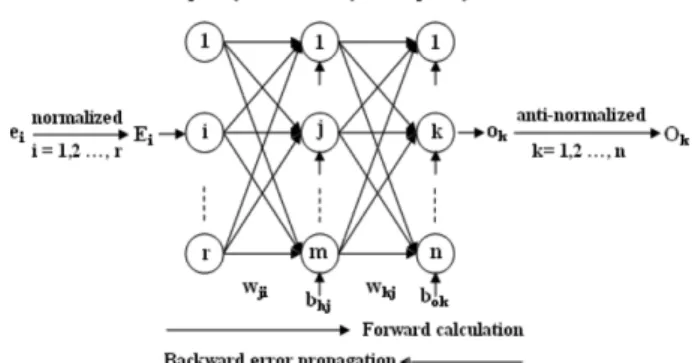
ANN consists of an input layer, a hidden layer, an out- put layer and connections between them (Fig. 1). The for- ward calculation and backward error propagation are the two parts involved in its operation.9
The node numbers of input layer, hidden layer and out- put layer are r, m and n, respectively. Wji and wkj denote the input-hidden layer connection weight and the hidden- output layer connection weight. To ensure the convergence of the network, the inputs (ei) need to be normalized before entering the network. The normalized data are obtained from following expression:
(1)
Where ai and bi refer to the minimum and maximum of ei respectively.
The normalized data (Ei) pass from input layer to hid- den layer along connecting weights, then to output layer.
Firstly, the node in hidden layer sums the weighted data from input layer plus a bias (bhj) then applies a transfer function to the sum as given by (for node j of the hidden
layer):
(2)
Where zj is the output of node j of the hidden layer. The sigmoid transfer function is adopted:
(3)
Secondly, it propagates the zj through outgoing connec- tions to the nodes of the output layer where it undergoes the same process as given by (for instance outputs zj of the hidden layer fed to node k of the output layer gives the output ok):
(4)
The pure linear expression is used as transfer function:
(5) The output of the network is produced by anti-normaliz- ing the ok:
(6)
Where ck and dk refer to the minimum and maximum of ( is the desired output) respectively. This process is called forward calculation.
The weights and bias are iteratively adjusted by prop- agating error signals backward along the connecting path- way until the output values of the network are close to the desired ones. The error signal of node k of the output layer is given by:
(7)
The δk is used to calculate the error signal of node j of the hidden layer:
(8)
This process is called backward error propagation. The ANN using this kind of algorithm is known as back prop- agation ANN (BP-ANN).
Strategies Suggested for Artificial Neural Network (1) There are seven variables involved in describing the liquid-liquid equilibrium data of hydrocarbon-water sys- tems in the state of vapour-liquid-liquid equilibrium: four Ei=(ei–ai)/ b( i–ai); i 1 2 … r= , , ,
zj fh wji
i 1=
∑
r ⋅Ei+bhj⎝ ⎠
⎛ ⎞; j 1 2 … m= , , ,
=
fh( ) 1/ 1 ex = ( + –x)
ok fo wkj
j 1=
∑
m ⋅zj+bok⎝ ⎠
⎛ ⎞; k 1 2 … n= , , ,
=
fo( ) xx =
Ok=ok(dk–ck) c+ ; k 1 2k = , , ,… n Oˆk Oˆk
δk=(Ok–Oˆk) d⋅( k–ck); k 1 2= , , ,… n
δj= wkj
k 1=
∑
n ⋅δk⎝ ⎠
⎛ ⎞ f⋅ h′ wji
i 1=
∑
r ⋅Ei+bhj⎝ ⎠
⎛ ⎞; j 1 2 … m= , , ,
Figure 1. The structure of artificial neural network.
intensive state properties (equilibrium temperature, equi- librium pressure and the mole fractions of hydrocarbon in two coexisting liquid phases) and three pure component properties of hydrocarbon (critical temperature, critical pres- sure and acentric factor). In this work, the equilibrium tem- perature and three pure component properties were selected as the input variables of the network. The mole fraction of hydrocarbon in hydrocarbon-rich phase (X1) and that in water-rich phase (Y1) were the output variables. The choice of the input and output data is based on the phase rule and the practical need to describe the four binary systems by only one ANN model. Table 1 lists the pure component propertiesused in this work.
It should be pointed that the equilibrium pressure has not been considered in the correlation using activity coef- ficient modelbecause the activity coefficient model excludes the pressure from its variables. Similarly, the equilibrium pressure was not selected as the variable of ANN model for the purpose of parallel comparision between the dif- ferent models.
(2) Due to the high asymmetry, the mutual solubilities between hydrocarbon and water are extremely low. The mole fractions of hydrocarbon in water-rich phase (Y1) range from 10−5 to 10−4 approximately. The direct corre- lation by means of the ANN model could produce poor results (it has been tested by author). In order to improve the correlation accuracy, the experimental data of Y1 were magnified with an appropriate multiple and then applied to correlation in this work. The correlated data of Y1 need to be reduced with the same multiple so that it can cater to the experimental data. This multiple was taken as 100 times which is proved to be suitable for improving the cor- relation accuracy of Y1.
(3) Only if the inputs of the network are within a certain interval (the most common interval is 0−1) can the sig- moid transfer function employed by ANN show an obvi- ous gradient, which ensures that the network can yield an acceptable convergence rate. Therefore, the inputs of the network need to be normalized (formula (1)). In view of the fact that the acentric factors of most substances belong to the interval of 0−1, the acentric factor, which was selected
as one of the inputs in this work, need not to be normal- ized.
On the other hand, the outputs of the network are lim- ited to a certain range because the sigmoid transfer function is a saturated function. In order to agree with the experimental data, the outputs of the network are usually obtained by anti-normalizing that of the output layer nodes (formula (6)).
It is well known that the mole fractions, which were selected as the outputs in this work, vary from 0 to 1 and can not be other values (it’s exactly the same as the range of the sig- moid function). For this reason, the anti-normalization was not adopted in this work. That is to say, the output of the network is equal to that of the output layer nodes:
(9) It should be noted that the error signal of the output layer nodes will be accordingly modified as follows:
(10) RESULTS AND DISCUSSION
(1) The above strategies were implemented in a pro- gram (made using delphi 6.0) for ANN modelling of the liquid-liquid equilibrium data of four hydrocarbon-water systems. The input layer of network is set with 4 nodes denoting the equilibrium temperature (T), the critical tem- perature (Tc), the critical pressure (Pc) and the acentric fac- tor (ω) of hydrocarbon respectively. The output layer has 2 nodes representing the mole fraction of hydrocarbon in hydrocarbon-rich phase (X1) and that in water-rich phase (Y1) respectively.
In this program, the error function is defined as follows:
RMS = (11)
Where N refers to the total number of data points. The basic principle for determining the node number of the hidden layer is to ensure that the error function can meet the following requirement:
RMS≤ error (12)
Where error is the control value for the termination of the program. The following steps are utilized to determine the error and the node number of the hidden layer:
1. The node number of the hidden layer can be roughly preset according to the personal experience. The weights and bias, which are the parameters of the network, are ran- domly initialized in the range (−0.5−0.5) by the program.
Ok=ok; k=1 2, , ,… n
δk=Ok–Oˆk; k 1 2= , , ,… n
0.5 [(X1cal–X1exp)i2+(Y1cal–Yexp1 )i2]
i 1=
∑
N⋅ Table 1. Pure component properties used in this work
Component Critical temperature (K)
Critical pressure (MPa)
Acentric factor
N-butane 425.40 3.797 0.193
Isobutane 408.10 3.648 0.176
Benzene 562.16 4.898 0.211
Toluene 591.79 4.104 0.264
2. The error is an important value due to its close relation to the correlation accuracy and the convergence rate of the network. The correlation accuracy can be investigated from the RMS (the smaller RMS means the higher accuracy):
(RMS/N)0.5= (13)
The convergence rate of the network can be evaluated by the running time of the program. With the decrease of the error, the correlation accuracy will be improved but the convergence rate will be lowered (the reverse is also true).
The error can be determined on condition that both the correlation accuracy and the convergence rate are taken into account.
The node number of the hidden layer can be finalized with the determination of the error. In addition to meeting the requirement (formula (12)), similarly, the choice of the node number of the hidden layer should give consider- ation to the correlation accuracy and the convergence rate.
It is especially noted that the correlation accuracy here refers to the absolute deviation (AD) of each data point rather than the above-mentioned one depending on the
error. The AD, which can be conveniently observed by plotting the correlated and experimental data in one fig- ure, is adjusted by changing the node number of the hid- den layer. The following expressions are used to calculate the ADX1 and ADY1:
ADX1= (14)
ADY1= (15)
The error and the node number of the hidden layer were identified as 0.000075 and 8 respectively according to the above procedure.
Table 2 shows the structure of the optimized ANN model. The weights and bias of the optimized ANN model are listed in Table 3, where wji is the input-hidden layer connection weight (8 × 4), wkj is the hidden-output layer connection weight (2 × 8), bhj is the bias of the hidden layer nodes (8) and bok is the bias of the output layer nodes (2).
(2) Table 4 lists the correlated results for the mole frac- tions based on the MPHC, NRTL and the proposed ANN models for selected systems. It can be seen that the aver- X1cal–X1exp
( )i2
Y1cal–Y1exp
( )i2
[ + ]/2N
i 1=
∑
N⎩ ⎭
⎨ ⎬
⎧ ⎫0.5
X1cal–X1exp
Y1cal–Y1exp
Table 2. Structure of the optimized ANN model
Type of network Input layer Hidden layer Output layer
BP ANN No. of nodes No.of nodes Transfer function No. of nodes Transfer function 4 (T, TC, PC, ω) 8 Sigmoid function 2 (X1, Y1) Pure linear function Table 3. Weights and bias of the optimized ANN model
Input layer-Hidden layer Hidden layer-Output layer
Weights Bias Weights Bias
wj1 wj2 wj3 wj4 bhj wlj w2j bok
−0.6143 −0.0748 0.4837 −0.2499 0.4434 0.5107 0.0442
0.1236 0.3121
−0.1137 0.1087 0.7787 −0.3846 0.2673 0.0827 1.1092
0.7868 −0.5715 0.1697 −0.4057 −0.2850 −0.4470 1.2953
−0.1689 −0.0743 −0.4805 −0.0079 −0.2143 0.2628 −0.5524
−1.0661 −0.5352 0.4700 0.3301 0.0846 −0.4745 −0.6319
1.7598 0.2443 0.7830 −0.2877 −0.9769 0.4224 −1.1451
−0.7019 −0.7441 −0.1991 0.3681 1.2382 0.7524 −0.9330
−0.4707 −0.2124 −0.3407 −0.3661 0.1013 0.2895 0.2494
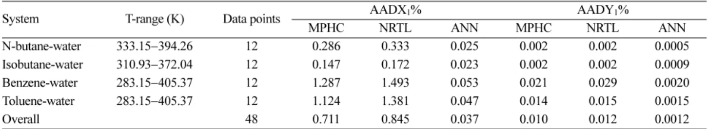
Table 4. Comparison of correlated results for the mole fractions of hydrocarbon-water phase equilibrium systems based on the different models
System T-range (K) Data points AADX1% AADY1%
MPHC NRTL ANN MPHC NRTL ANN
N-butane-water 333.15−394.26 12 0.286 0.333 0.025 0.002 0.002 0.0005
Isobutane-water 310.93−372.04 12 0.147 0.172 0.023 0.002 0.002 0.0009
Benzene-water 283.15−405.37 12 1.287 1.493 0.053 0.021 0.029 0.0020
Toluene-water 283.15−405.37 12 1.124 1.381 0.047 0.014 0.015 0.0015
Overall 48 0.711 0.845 0.037 0.010 0.012 0.0012
age absolute deviations (AAD) of the correlated mole fractions from experimental data3 are remarkably reduced by the ANN model than the MPHC and NRTL models. The AADX1 and AADY1 can be obtained from following expressions:
AADX1= (16)
AADY1= (17)
Where NP refers to the number of data points.
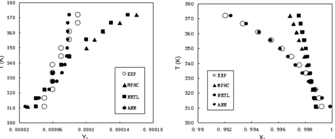
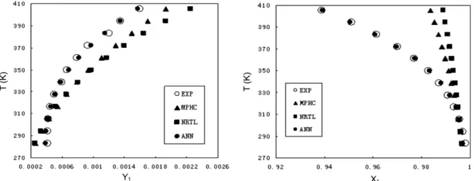
Simultaneously, the comparisons between the experi- mental and correlated data are plotted in Fig. 2 to 5. These figures show that the ANN model gives better description of the experimental data within the temperature range for which the model has been designed.
Furthermore, the measured result shows that the running of the program takes one minute or so, which means an acceptable convergence rate of the network.
(3) We must admit that due to its empiricism, ANN is inferior to the traditional thermodynamic models in terms of theoretical foundation, although it can yield satisfac- tory results for the phase equilibria of these binary hydro- carbon-water systems.
X1cal–X1expi
i 1= NP
∑
/NpY1cal–Y1expi/Np
i 1= NP
∑
Figure 2. Comparison of the correlated mole fractions of n-butane based on different models with experimental data under different temperatures.
Figure 3. Comparison of the correlated mole fractions of isobutane based on different models with experimental data under different temperatures.
CONCLUSION
A back propagation artificial neural network model was developed for simulation of the phase equilibria in four hydrocarbon-water systems. It does not require the binary interaction parameters, nor did the mixing rules as required by conventional methods. For further improving the cor- relation ability of ANN model, some reasonable strate- gies are put forward in terms of the network structure, the data processing, as well as the algorithm. Better results are achieved from the ANN model based on these ideas although the equilibrium data cover a large range of temperature.
This study also shows that ANN model could be developed for the phase equilibria for a family of hydrocarbon-water binaries, provided reliable experimental data are available, to be used in chemical engineering applications.
Acknowledgments. The publication cost of this paper was supported by the Korean Chemical Society.
REFERENCES
1. Huynh, D. N.; de Hemptinne, J. C.; Lugo, R.; Passarello, J. P.; Tobaly, P. Ind. Eng. Chem. Res. 2011, 50, 7467.
2. Fonseca, J. M. S.; von Solms, N. Fluid Phase Equilib.
2012, 329, 55.
3. Wang, L. S.; Guo, T. M. Chem. Eng. (China) 1996, 24, 59.
4. Riaz, M.; Yussuf, M. A.; Kontogeorgis, G. M.; Stenby, E.
H.; Yan, W.; Solbraa, E. Fluid Phase Equilib. 2013, 337, 298.
5. Panagiotopoulos, A. Z.; Reid, R. C. Prepr. Pap. Am. Chem.
Soc. Div. Fuel Chem. 1985, 30, 46.
6. Neau, E.; Escandell, J.; Nicolas, C. Ind. Eng. Chem. Res.
Figure 4. Comparison of the correlated mole fractions of benzene based on different models with experimental data under different tem- peratures.
Figure 5. Comparison of the correlated mole fractions of toluene based on different models with experimental data under different tem- peratures.
2010, 49, 7580.
7. Escandell, J.; Neau, E.; Nicolas, C. Fluid Phase Equilib.
2011, 301, 80.
8. Gebreyohannes, S.; Yerramsetty, K.; Neely, B. J.; Gasem, K. A. M. Fluid Phase Equilib. 2013, 339, 20.
9. Si-Moussa, C.; Hanini, S.; Derriche, R.; Bouhedda, M.;
Bouzidi, A. Braz. J. Chem. Eng. 2008, 25, 183.
10. Dehghani, M. R.; Modarress, H.; Bakhshi, A. Fluid Phase Equilib. 2006, 244, 153.
11. Mohammadi, A. H.; Richon, D. Ind. Eng. Chem. Res.
2007, 46, 1431.
12. Ketabchi, S.; Ghanadzadeh, H.; Ghanadzadeh, A.; Fallahi, S.; Ganji, M. J. Chem. Thermodyn. 2010, 42, 1352.
13. Faundez, C. A.; Quiero, F. A.; Valderrama, J. Q. Fluid Phase Equilib. 2010, 292, 29.
14. Lashkarbolooki, M.; Vaferi, B.; Rahimpour, M. R. Fluid Phase Equilib. 2011, 308, 35.
15. Safamirzaei, M.; Modarress, H. Fluid Phase Equilib. 2011, 309, 53.
16. Lashkarbolooki, M.; Vaferi, B.; Rahimpour, M. R. Fluid Phase Equilib. 2011, 308, 35.
17. Safamirzaei, M.; Modarress, H. Fluid Phase Equilib. 2011, 310, 150.
18. Bakhbakhi,Y. Expert Syst. Appl. 2011, 38, 11355.
19. Abedini, R.; Zanganeh, I.; Mohagheghian, M. J. Phase.
Equilib. Diff. 2011, 32, 105.
20. Zarenezhad, B.; Aminian, A. Korean J. Chem. Eng. 2011, 28, 1286.
21. Pahlavanzadeh, H.; Nourani, S.; Saber, M. J. Chem. Ther- modyn. 2011, 43, 1775.
22. Nami, F.; Deyhimi, F. J. Chem. Thermodyn. 2011, 43, 22.
23. Shokri, A.; Hatami,T.; Khamforoush, M. J. Supercrit. Fluids 2011, 58, 49.
24. Rohani, A. A.; Pazuki, Gh.; Abedini Najafabadi, H.; Seyfi, S.; Vossoughi, M. Expert. Syst. Appl. 2011, 38, 1738.
25. Lashkarbolooki, M.; Hezave, A. Z.; Ayatollahi, S. Fluid Phase. Equilib. 2012, 324, 102.
26. Hezave, A. Z.; Lashkarbolooki, M.; Raeissi, S. Fluid Phase Equilib. 2012, 314, 128.
27. Sinha, K.; Chowdhury, S.; Saha, P. D.; Datta, S. Ind. Crop.
Prod. 2013, 41, 165.
28. Mandal,S.; Jana, A. K. Int. J. Hydrogen Energy 2013, 38, 1244.
29. Lashkarbolooki, M.; Shafipour, Z. S.; Hezave, A. Z.; Far- mani, H. J. Supercrit. Fluids 2013, 75, 144.