Vol. 12, No. 8 pp. 3384-3390, 2011
Domain Decomposition Method for Elasto-Plastic Problem
Byung-Kyu Bae
1and Joon-Seong Lee
2*1Dept. of Mechanical Engineering, Graduate School, Kyonggi University
2Dept. of Mechanical System Engineering, Kyonggi University
탄소성문제 적용을 위한 영역분할법
배병규
1, 이준성
2*1경기대학교 대학원 기계공학과, 2경기대학교 기계시스템공학과
Abstract This paper describes a domain decomposition method of parallel finite element analysis for elasto-plastic structural problems. As a parallel numeral algorithm for the finite element analysis, the authors have utilized the domain decomposition method combined with an iterative solver such as the conjugate gradient method. Here the domain decomposition method algorithm was applied directly to elasto-plastic problem. The present system was successfully applied to three-dimensional elasto-plastic structural problems.
요 약 본 논문은 탄소성 구조해석을 위한 병렬유한요소해석에 필요한 영역분할법에 대해 제시하고 있다. 유한요소
해석을 위한 알고리즘으로서 CG방법과 결합한 영역분할법을 이용하였다. 적용된 영역분할법은 탄소성문제를 해석하
는데 직접적으로 사용되어 지며 효용성 검토를 위해 3차원 탄소성 구조문제에 적용하여 해석해 본 결과 높은 병렬효
과를 발휘함을 알 수 있었다.
Key Words : Finite Element Analysis, Domain Decomposition Method, Elasto-Plastic Analysis
*Corresponding Author : Joon-Seong Lee([email protected])
Received June 01, 2011 Revised (1st July 05, 2011 2nd July 12, 2011) Accepted August 11, 2011
1. Introduction
The demand for large scale analysis is mainly from nonlinearity which cause longer time to get result. For large scale three dimensional nonlinear structural problems[1], direct solvers entail memory and CPU requirements that rapidly overwhelm even the largest hardware resource currently available.
The elasto-plastic finite element method[2-4] is one of the most powerful tools for fracture mechanics analysis of materials of high ductility. In practical applications of that method, however, the following two problems arise to obtain accurate and reliable results.
The first problem is that the elasto-plastic finite element method requires a huge amount of computer memory. In fracture mechanics analysis of practical
structures, a very fine three dimensional finite element mesh is required to model a whole structure as well as a postulated surface flaw. The second problem is a huge amount of computation time caused due to a number of incremental calculations.
To handle these problems, strongly demanded is the development of the new finite element method algorithms which save memory as well as computation time, that is, the parallel finite element method based on the domain decomposition method(DDM)[5-7].
As a parallel numerical algorithm for the finite element analysis, the present authors have proposed the domain decomposition method combined with an iterative solver[3]. In this method, a whole domain to be analyzed is fictitiously divided into a number of subdomains without overlapping, and the finite element analyses of
each subdomain is performed in parallel. And the DDM algorithm can be applied to incremental formulations of elasto-plastic problems.
2. CG Algorithm for DDM
To explain its theory, let us consider an elastic problem concerning a domain Ω, as shown in Fig. 1.
Here, is the traction force applied on the boundary
, the body force applied in the domain Ω, and the prescribed displacement on the boundary .
[Fig. 1] Analysis domain
Fundamental equations of this elastic problem are summarized in an infinitesimal displacement mode as follows:
in Ω (1)
in Ω (2)
in Ω (3) on (4)
on (5)
where i, j take the value 1 to 3, is a displacement vector, a strain tensor, stress tensor, Ci,jmn a coefficient tensor of the Hooke's law and an outer normal vector on the boundary , respectively. (),j
denotes the first order derivative with respect to the coordinate .
The above variational from is equivalent to the
following minimization problem which finds the displacement function u which is a stationary point of the energy functional :
(6)
[Fig. 2] Analysis domain split into subdomain
As shown in Fig. 2, after dividing domain Ω into Nd
subdomains, ≤ ≤
with being the interface between and , solving the above problem is equivalent to finding the displacement functions
which are stationary points of the energy functional:
′
(7)
with additional conditions on the interface boundary
:
on (8)
on (9)
where the superscripts ()(d) designate variable defined in the subdomains .
Defining the positive definite and symmetric operator A:
(10) where
on (11)
the CG algorithm for solving equation[2] is summarized as follows:
Step 0: Initialization
: arbitrarily given (12)
(13)
(14)
The of equation (13) is obtained from the traction forces on which are calculated by solving equations (1)~(5) in each subdomains with following constraint:
on (15)
Step 1: Steepest descent
(16)
where
(17)
Step 2: Calculation of the new descent direction
(18)
(19)
where
(20)
The of equation (17) and (18) is obtained from the traction forces on which are calculated by solving the following equations:
in Ω(d) (21)
on (22)
on (23)
on (24)
Step 3: Judgment of convergence
If has not converged yet, return to step 1 by setting n to be n+1. Here the convergence criterion is defined as:
≺ (25)
in which the maximum component of force imbalance along the interface boundary, i.e. residual value, is monitored.
3. DDM algorithm for Elasto-Plastic Problem
The domain decomposition method(DDM) can be applied directly to incremental formulations of elasto- plastic problem based on the J2 flow theory[3]. With the incremental method, force or displacement of boundary condition is divided among each incremental step and in each step, the nonlinear problem can be solved as a linear problem to which the DDM algorithm is applied.
For nonlinear problems, the stress-strain equation, i.e.
the constitutive equation is written as follows:
∆
′
∆ (26)where {△σ} and {△ε} are the stress and strain increment, [D'(σ)] is the tangential matrix, respectively.
At each incremental step, the following incremental formulations are used.
(27)
(28)
(29)
(30)
Considering these equations, the stiffness equation is
described as follows:
′
∆ ∆ (31) (32)
where [K'] is the tangential stiffness matrix and {R}(i-1) is the residual vector which indicate imbalance at step (i-1).
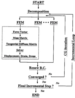
[Fig. 3] Flow chart of DDM for elasto-plastic analysis
The present DDM was applied to solve these equations. The DDM algorithm for elasto-plastic problem is shown in Fig. 3. With such a algorithm, the number of iterations of the DDM in each of the incremental steps is expected to reduce by using the result in the incremental step as the initial value of the iterative calculation in the current step.
4. Analysis of Test Model
In order to evaluate the result performed by the present parallel finite element method system, its solution, the stress-strain curve calculated by the present system, which is abbreviated as 'DDM', are compared with those by the commercial sequential finite element method system,
MSC/NASTRAN, which is abbreviated as 'FEM'.
'DDM' and 'FEM' are applied to the FE analysis of a cubic structure subject to uniform tension. The structure was modeled with 10,368 4-node tetrahedral elements, and the total DOF was 6,591. In the case of analysis of 'DDM', the whole structure was divided into 27 subdomains and each subdomain consists of 384 elements as shown in Fig. 4.
Table 1 shows the maximum and mean value of the errors of displacement and stress respectively given by 'DDM' relative to 'FEM'. Here, the displacement and stress, denoted
as and
, respectively, are defined as follows:
(33)
(34)
where
are the displacement values of axis x, y, z,
are the stresses of axis x, y, z and
are the shear stresses.[Fig. 4] Cubic model with decomposition
[Table 1] Error of DDM for FEM
Displacement Stress Max. Error 1.03 % 1.51 %
Mean Error 0.30 % 0.42%
With this system, we can divide the model into any number of subdomains. Then how to decide the division number is important for performance.
For simplicity, a cubic model shown in Fig. 4 is used here to estimate the computational time. Each axis of the model is now divided by N with isoparametric 8-noded elements, therefore, the domain of the model is divided into N3 elements and the total number of nodes is equivalent to (N+1)3. Each axis is then divided into subdomains by d, and therefore, the total number of subdomains is equivalent to d3 and each subdomain consists of (N/d)3 elements and (N/d +1)3 nodes, DOF of which, Dsubdomain, is (N/d +1)3 × 3. The total number of interface DOF, Dinterface, on the other hand amounts to approximately (N2×d×3).
Now the computational time of the FEM analysis of each subdomain, Tdomain and the total number of CG iterations Niteration can be evaluated as follows:
× (35)
× × (36)
where
and
are function of DOF of each subdomain and DOF of interface, respectively.Using
and
, ignoring communication, total computational time Ttotal can be described as follows:× ×
× × (37)
Unfortunately, those functions are unknown but it can be only estimated in a rough fashion. For
, with a direct solver, the main part of FEM analysis is the factorization of matrix part and forward and backward elimination part. The order of operation times of these calculation are O(N3) and O(N2), respectively, where N is DOF of problem. Here, for simplicity,
is defined as a quadratic function of Dsubdomain.For
, from the CG algorithm for matrix solution, it is known that the number of iterations is linear to the square root of DOF and its coefficient depends on the condition number of the matrix.Using these assumptions,
and
are described as follows:
(38)
(39)where a, b, c, d and e are all coefficients.
To find out these coefficients, the total computational time can be estimated. To determine them, some numerical experimentations are performed here. For some sets of N and d, analyses of the DDM are performed and
and
are evaluated.[Table 2] Computational time and CG iterations
N d Dsubdomain Dinterface fi fc Ttotal
8 2 375 583 0.58 20 92.8
8 4 81 1,359 0.04 25 66.8
12 3 375 2,406 0.58 26 407.2
12 4 102 3,315 0.17 29 329.7
24 4 1,092 14,367 4.10 43 11386.4 24 6 375 21,975 0.58 47 5888.2 24 8 192 28,175 0.17 53 4613.1 24 12 81 36,927 0.04 58 4009.0
The results of these numerical experimentations which are performed by only on workstation, Sun SS(50MHz), are shown in Table 2. In this assumption, since communication time is avoided, one processor is used for all execution of the DDM without communication.
For example, the total computation time Ttotal were estimated and plotted against division number d in Fig. 5 As shown in this figure, there exists one division number d which minimize the total computation time.
Fig. 6 shows the stress-strain curves obtained from 'DDM' and 'FEM'. It is shown that these curves are identical except near the yield point. In those algorithms, each size incremental step is taken differently. While the regular interval is taken in the whole computation in 'FEM', the first interval is jumped to of the yield point to avoid iterations in the elastic region which can be solved by one step. This is why those curves do not match with each other near the yield point.
[Fig. 5] Computational time vs division number
[Fig. 6] Stress-strain curve of elasto-plastic analysis As a large scale problem, the same structure was modeled with 46,656 isoparametric 8-noded elements with the total 151,959 d.o.f. The whole structure was then divided into 216 subdomains each with 216 elements.
This problem was solved by WSC, the variations of the residual value, defined in equation (25), against the number of the CG iterations of 6 incremental steps are shown in Fig. 7. It is shown here that the residual values decrease with the increase of the number of iterations in each incremental step.
[Fig. 7] Residual vs number of iterations for elasto-plastic analysis
5. Conclusions
The parallel finite element system based on the domain decomposition method and conjugate gradient method was successfully developed in the present study. This DDM system was applied to incremental formulations of elasto- plastic problems and demonstrated that this parallel finite element method system is useful for such problems as well as linear problems.
References
[1] J. S. Lee, "Automated CAE System for Three-Dimensional Complex Geometry", Doctoral Thesis, The University of Tokyo, 1995.
[2] G. Yagawa, S. Yoshimura, "Finite Element Method", BaePungKwan Press, pp. 193-207, 2001.
[3] S. Moaveni, "Finite Element Analysis", Prentice Hall, Inc., 1999.
[4] Choi, J. B., Park, Y. J., Ko, H. O., Chang, Y. S., Kim, Y. J. and Lee, J. S., "Parallel Procecess System and Its Application to Flat Display Modules Impact Analysis", Proceedings of the 7th World Congress on Computational Mechanics, pp. 16-22, 2006.
[5] J. S. Lee, R. Shioya, E. C. Lee and Y. C. Lee,
"Parallel Finite Element Analysis System Based on Domain Decomposition Method", Journal of the Computational Structural Engineering Institute of Korea, Vol. 22, No. 1, pp. 35-44, 2009.
[6] J. F. Thompson, B. K. Soni and N. P. Weatherill,
"Grid Generation", CRC Press, pp. 12-25, 1998.
[7] Nguyen, D. T. and Al-Nasra, M., "An Algorithm for Domain Decomposition in Finite Element Analysis", Computer and Structures, Vol. 39, No. 3, pp. 277-289, 1991.
Acknowledgement
The authors thank Professor R. Shioya for providing relevant advice.
Byung-Kyu Bae
[Regular member]• 2010 : Dept. of Mechanical Eng, Kyonggi University(B.S)
• 2010~now : Dept. of Mechanical Eng, Kyonggi University(M.S)
<Research Interests>
Structural Analysis, Fatigue Assessment, Integrity Evaluation
Joon-Seong Lee
[Regular member]• 1988 : Dept. of Mechanical Eng, SungKyunKwan University(M.S)
• 1988~1991 : Professor in Dept.
of Mechanical Eng. of Korea Military Academy
• 1995 : Dept. of Mechanical Eng, The University of Tokyo(Ph.D)
• 1996~now : Professor in Dept.
of Mechanical Eng, Kyonggi University
<Research Interests>
Optimal Design, Neural Network, Automatic Mesh Generation