Tensor framelet based iterative image reconstruction algorithm for low-dose multislice helical CT

(1)

Tensor framelet based iterative image

reconstruction algorithm for low-dose

multislice helical CT

Haewon NamID1, Minghao Guo2, Hengyong YuID3, Keumsil Lee4, Ruijiang Li5, Bin Han5, Lei Xing5, Rena Lee6, Hao Gao7*

1 Department of Liberal Arts, Hongik University, Sejong, Republic of Korea, 2 School of Biomedical Engineering, Shanghai Jiao Tong University, Shanghai 200240, China, 3 Department of Electrical and Computer Engineering, University of Massachusetts, Lowell, Massachusetts 01854, United States of America, 4 Department of Radiology, Stanford University, Stanford, California 94305, United States of America, 5 Department of Radiation Oncology, Stanford University, Stanford, California 94305, United States of America, 6 Department of Radiation Oncology, Ewha Womans University, Seoul, Korea, 7 Department of Radiation Oncology, Emory University, Atlanta, GA 30322, United States of America

*[email protected]

Abstract

In this study, we investigate the feasibility of improving the imaging quality for low-dose mul-tislice helical computed tomography (CT) via iterative reconstruction with tensor framelet (TF) regularization. TF based algorithm is a high-order generalization of isotropic total varia-tion regularizavaria-tion. It is implemented on a GPU platform for a fast parallel algorithm of X-ray forward band backward projections, with the flying focal spot into account. The solution algo-rithm for image reconstruction is based on the alternating direction method of multipliers or the so-called split Bregman method. The proposed method is validated using the experi-mental data from a Siemens SOMATOM Definition 64-slice helical CT scanner, in compari-son with FDK, the Katsevich and the total variation (TV) algorithm. To test the algorithm performance with low-dose data, ACR and Rando phantoms were scanned with different dosages and the data was equally undersampled with various factors. The proposed method is robust for the low-dose data with 25% undersampling factor. Quantitative metrics have demonstrated that the proposed algorithm achieves superior results over other exist-ing methods.

Introduction

X-ray computed tomography (CT) has been one of the most widely used medical imaging techniques since Hounsfield invented the first commercial medical X-ray machine in 1972 [1]. The Helical CT was first invented by I. Mori [2] in the late 1980s and was developed by W. Kalender [3] in the 1990s. The number of detector rows has been increased to achieve larger volume coverage with a reduced scan time and improved z-resolution. The 8-slice CT system was first introduced in 2000, Siemens SOMATOM Definition scanner has 64-slice rows for up

a1111111111 a1111111111 a1111111111 a1111111111 a1111111111 OPEN ACCESS

Citation: Nam H, Guo M, Yu H, Lee K, Li R, Han B, et al. (2019) Tensor framelet based iterative image reconstruction algorithm for low-dose multislice helical CT. PLoS ONE 14(1): e0210410.https://doi. org/10.1371/journal.pone.0210410

Editor: Qinghui Zhang, North Shore Long Island Jewish Health System, UNITED STATES Received: September 10, 2018 Accepted: December 21, 2018 Published: January 11, 2019

Creative Commons Attribution License, which permits unrestricted use, distribution, and reproduction in any medium, provided the original author and source are credited.

Data Availability Statement: All relevant data are within the manuscript and its Supporting Information files.

Funding: H. Nam was supported by the Basic Science Research program through NRF (#2015R1C1A2A01054731) of Korea funded by the ministry of Education Science and Technology. L. Xing is supported partially by NIH/NIBIB 1R01 EB-016777. R. Lee was supported by the Korea Institute for Advancement of Technology (KIAT) grant funded by the Korea government (Ministry of Trade, Industry and Energy, No.0001723).

(2)

to 128-channel data acquisition, and the Toshiba Aquilion ONE ViSION, which has 320-slice rows for generating 640 slices, was brought out in 2013.

Helical CT reconstruction algorithms can be categorized into two groups: Analytic recon-struction and iterative algorithm. An analytic reconrecon-struction can be sub-divided into exact and approximate reconstruction methods. The Feldkamp-Davis-Kress algorithm (FDK) is a well-known approximate analytic reconstruction algorithm [4] and it can be generalized for helical scan trajectories [5–7]. However, FDK generates helical artifacts due to data insuffi-ciency. A conventional filtered backprojection (FBP) algorithm can be implemented with data interpolation [8] to soften helical artifacts, but this may generate another type of artifact caused by data approximation. In 2002, Katsevich introduced an exact FBP-type reconstruction algo-rithm based on the PI-line and Tam-Danielsson window [9–11]. Details for the numerical implementation of the Katsevich algorithm are given in [12,13]. An alternative derivation of the Katsevich algorithm is provided by Chen [14]. Meanwhile, another exact method of back-projection-filtration (BPF) has been developed by Zou and Pan [15], and these ideas have inspired several subsequent exact reconstruction methods [16–20].

Katsevich-type algorithms are based on exact analytic theory, and thus it is sensitive to the noisy projection data. To overcome these noise sensitivity, many researchers have studied iter-ative reconstruction algorithms [21,22] by formulating the image reconstruction as an optimi-zation problem based on versatile CT models. The Algebraic Reconstruction Technique (ART) [1,23] and Simultaneous Algebraic Reconstruction Technique (SART) [24] are two of the most popular methods in the early stage of iterative reconstruction algorithms. Iterative reconstruction algorithms are based on a mathematical minimization which seeks the best approximate solution. They have greater flexibility, and thus are robust against noise. A regu-larization term, such as Tikhonov or total-variation (TV) regularizer, can be added to the cost function for noise and artifact reduction. Compared with analytic reconstruction algorithms, iterative reconstruction algorithms work well even with insufficient or low-dose data. However a significant disadvantage of iterative reconstruction is its high computational cost, particularly for helical CT scans, which contain a huge amount of data. Thanks to recent advances in com-puting hardware, iterative reconstruction is emerging for helical CT [21,22,25,26]. Nuyts et al. [22] investigated the superiority of iterative reconstruction compared to non-iterative methods for a helical CT system. They concluded that iterative reconstruction improved the axial resolution. Thibault et al. [21] presented a Bayesian iterative reconstruction algorithm for multislice helical data, they showed improved high contrast spatial resolution and signal-to-noise ratio relative to analytic methods. Yu and Zeng [26] developed a TV-based iterative algo-rithm and applied it to a limited-angle inverse helical CBCT reconstruction for C-arm system.

In this article, we propose an iterative reconstruction algorithm to improve multi-slice heli-cal CT based on tensor framelet (TF) [27,28] regularization. The method belongs to a spar-sity-regularized model-based iterative reconstruction, which is inspired by compressive sensing [29,30]. To name a few: Sidky et al. develops a TV-based iterative method for sparse-view and limited-angle reconstruction [31]; Chen et al. proposes the so-called PICCS method for the dynamic CT problem [32]; Yu and Wang studies the sparsity-regularized method for interior tomography [33]; Gao et al. proposes a rank-sparsity decomposition method for dynamic CT [34] and spectral CT [35]; Jia et al. studies tight frame regularization for cone-beam CT image reconstruction [36]; Xu et al. develops a dictionary learning-based image reconstruction method for dose reduction [37].

This paper is organized as follows: Section II provides the materials and method details, including the minimization problem, TF regularization, optimization algorithm for iterative multislice helical CT image reconstruction, and experimental details. Section III presents the validation of the proposed method for low-dose multislice helical CT in comparison with

Competing interests: The authors have declared that no competing interests exist.

(3)

FDK, the Katsevich and TF algorithms, with low-dose and sparse-view data. Section IV sum-marizes this work.

Materials and methods

Minimization problem

The mathematical formulation of an iterative CT reconstruction can be expressed by a least-square minimization problem as

x ¼ arg min x 1 2kAx yk 2 2þ lRðxÞ; ð1Þ

where x is the three-dimensional image to be reconstructed with given projection data y and the projection matrix A. The first term indicates the data fidelity in theL2-norm. The second term consists ofR(x) as a regularization function with regularization parameter λ. For exam-ple, the TV norm is a popular regularization choice for sparsity-based CT image reconstruc-tion [31,32].

In this paper, we solveEq (1)with the given data y from the multislice helical CT system. The projection matrix A contains the helical geometry with the flying focal spot [38]. For the forward projection A and its adjoint AT, parallelized algorithms with an infinitely narrow beam are used with GPU implementation [39].

Tensor framelet regularization. Consider a 3D image x as a tensor, x ¼ fxijk;i � Nx; j � Ny; k � Nzg

wherexijkis the (i, j, k)-th voxel in three-dimensional image space, Nx,Ny, andNzare the

num-ber of voxels in thex, y and z–axis respectively. We define xx, xy, and xzas 1D unfolded

matri-ces of x along thex, y, and z–axes, respectively. The TF transform is constructed using the standard 1D framelet transform [40], e.g., the 1D piecewise linear tight frame with the follow-ing refinement masks.

o0 ¼ 1 4½1 2 1�; o1 ¼ ffiffiffi 2 p 4 ½1 0 1�; o2¼ 1 4½ 1 2 1�:

The operatorω0is an averaging operator, and the two other operatorsω1andω2are the first

and second differential operators, respectively. Note thatω0smoothes the image, whileω1and

ω2enhance the edges. Define

M_jx ¼ 1ffiffiffi 3 p o_j� x_x o_j� x_y o_j� x_z 2 6 6 6 4 3 7 7 7 5; 8j ¼ 0; 1; 2;

where�_{denotes the convolution operator. The TF regularization function W and its adjoint} WTare respectively defined as below.

Wx ¼ ½M0x; M1x; M2x� T ; ð2Þ and WTy ¼ MT0ðM0xÞ þ M T 1ðM1xÞ þ M T 2ðM2xÞ; for y ¼ Wx: ð3Þ

(4)

kMjxk1¼ ffiffiffiffiffiffiffiffiffiffiffiffiffiffiffiffiffiffiffiffiffiffiffiffiffiffiffiffiffiffiffiffiffiffiffiffiffiffiffiffiffiffiffiffiffiffiffiffiffiffiffiffiffiffiffiffiffiffiffiffiffiffiffiffi jo_j�xxj 2 þ jo_j�xyj 2 þ jo_j�xzj 2 q

, for allj = 0, 1, and 2. TF transform W is left invertible and WTW =I, by the simple calculation [27]. Ifλ0= 0,λ16¼ 0, andλ2= 0, kWxk1

corresponds to the isotropic TV norm of x. In other words, TF regularization is a high-order generalization of TV.

The TF transform W can be extended to the multilevel by diluting the masks to ol

isuch that ol 0 ¼ 1 4½1 0 � � � 0|fflffl{zfflffl} 2l 1 2 0 � � � 0 |fflffl{zfflffl} 2l 1 1�; ol 1 ¼ ffiffiffi 2 p 4 ½1 0 � � � 0|fflffl{zfflffl} 2l 1 0 0 � � � 0 |fflffl{zfflffl} 2l 1 1�; ol 2 ¼ 1 4½ 1 0 � � � 0|fflffl{zfflffl} 2l 1 2 0 � � � 0 |fflffl{zfflffl} 2l 1 1�:

Similar to the uni-level TF, definexl_{¼ o}l

0�xl 1, x 0 = x and Ml jx l_¼ 1_ffiffiffi 3 p ol j�xlx ol j�x l y ol j�x l z 2 6 6 6 6 4 3 7 7 7 7 5; 8j ¼ 0; � � � ; 2; 8l ¼ 1; � � � L:

Then TF transform W with levelL is

Wx ¼ M1 1x 1 M1 2x 1 |fflfflfflfflfflfflffl{zfflfflfflfflfflfflffl} 1st level � � � Ml 1x l _Ml 2x l |fflfflfflfflfflfflffl{zfflfflfflfflfflfflffl} l th level � � � xL _ML 1x L _ML 2x L |fflfflfflfflfflfflfflfflfflffl{zfflfflfflfflfflfflfflfflfflffl} L th level 2 6 4 3 7 5; ð4Þ

and its adjoint WTis defined as

WT_ð_{yÞ ¼ x}L_þX L l¼1 X2 j¼1 Ml jx l_; _for _{y ¼ Wx} ð5Þ

Similarly, Eqs(4)and(5)are a generalization of TV to multilevel, and it keeps the framelet features such as WT(Wx) = x. With the TF regularization,Eq (1)becomes

x ¼ arg min x 1 2kAx yk 2 2þ lkWxk1: ð6Þ

The TF regularization term is defined as the isotropic shrinkage TF norm [27]: lkWxk1¼ XL l¼1 X2 j¼1 l_l;jkMl jx l_k 1þ lL;0kx L_k 1: ð7Þ

Optimization algorithm. The TF regularization(7)is the summation ofL1-norm. To

solve the non-differentiableL1minimization problem(6), we choose the alternating direction

method of multipliers (ADMM) [41] or the so-called Split Bregman method [42]. In general it is difficult to solve theL1-regularized minimization problem because it has non-differentiable

(5)

variables d, and v.Eq (6)becomes x ¼ arg min x; d; vlkdk1þ 1 2kAx yk 2 2þ m 2kWx d þ vk 2 2; ð8Þ

which can be split into three steps: • Step 1:xnþ1_¼_{arg min}

x 1 2kAx yk 2 þm 2kWx d n þvn_k2 2

• Step 2:dnþ1¼arg mindkdk1þ m 2kWx

nþ1 _{d þ v}n_k2 2 • Step 3: vn+1= vn+ Wxn+1− dn+1

Because of the decoupled form, step 1 is the sum of two differentiableL2-norm terms. Thus,

we can efficiently solve it from its optimal condition by the conjugate gradient method. Note that TF is more computationally efficient than TV due to WTW =I. Step 2 can be solved effi-ciently using the TF shrinkage formula [28]. Step 3 is in its explicit form, thus it is easy to implement.

Experiments

Data acquisition. The multislice helical CT reconstruction quality was evaluated using

the American College of Radiology (ACR) CT accreditation phantom (Data Spectrum Corpo-ration. Model: ECT/DLX/P) and the Rando phantom. Siemens SOMATOM Definition 64-slice helical CT scanner was used to generate the helical CT projection data. Details of the scan parameters for ACR phantom were as follows: Various voltage parameters with effective mAs, CTDIvol, and DLP are described inTable 1. For every voltage level, there was a 3.05s

scan time, 0.5s gantry rotation time, and 64�0.6 mm collimation with z-flying focal spot. The helical pitch is set to bep = 1, with 2304 projections per rotation. Image volume resolution is: 2 mm slice thickness and 0.9766 × 0.9766 mm2axial resolution. The whole image volume has 512× 512 × 88 voxels. A 21.6 cm inside diameter cylindrical ACR phantom is used. Parameter details for the Rando phantom scan were as follows: 120kV with 350 effective mAs are used. There was a 17s scan time and 20�_{0.6 mm collimation with z-flying focal spot. The helical}

pitch is set to bep = 1, with 4608 projections per rotation. Image volume resolution is: 4 mm slice thickness and 0.9766× 0.9766 mm2axial resolution. The whole image volume has 512× 512 × 53 voxels.

Quantitative metrics. To evaluate the performance of the proposed algorithm

quantita-tively in comparison to FDK and the Katsevich algorithm, four different quantitative metrics are selected. The Universal Quality Index (QUI) measures the intensity similarity between the reconstructed and true images. Image noise is measured by Signal-to-Noise Ratio (SNR) and Contrast-to-Noise Ratio (CNR). These two metrics quantify the noise level of the recon-structed images. The Modulation Transfer Function (MTF) is used to evaluate the resolution of the reconstructed images.

Image similarity—Universal Quality Index (UQI). The Universal Quality Index (UQI)

[43] was measured to evaluate the similarity between the reconstructed and true images. We considered the image from the scanner to be the true image. Given the ROI within the recon-structed and true images, the associative mean of the imageμ, the variance and covariance of μ with the true imageμtrueover the ROI are denoted as �m,σ

2

, and Cov(μ, μtrue), respectively.

The definition of UQI is given as

UQI¼4Covðm; mtrueÞ

s2_{þ s}2 true � m � �mtrue � m2_{þ �}_m2 true :

(6)

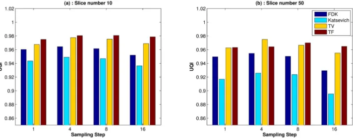
The UQI measures the intensity similarity between two images, and its value ranges [0, 1]. A UQI value close to 1 indicates a better level of similarity between the reconstructed and true images. We chose two ROIs: The whole ACR phantom body on slices 10 and 50. We calculated the UQI scores for all three methods under comparison.

Image noise—SNR and CNR. To evaluate the quantitative noise level of the reconstructed

images, we chose two different metrics, SNR and CNR. The definitions are as follows.

SNR¼m�ROI

sROI

CNR¼ j�mROI m�ROIairj

ffiffiffiffiffiffiffiffiffiffiffiffiffiffiffiffiffiffiffiffiffiffiffiffiffiffiffi s2 ROIþ s 2 ROIair q

whereσROIand sROIairrefer to the standard deviations and �mROIand �mROIairrefer to the

mean pixel value in a ROI inside and the background of the phantom, respectively. We chose four Regions Of Interest (ROI) to compare the reconstructed images from all three methods with that from the scanner. For convenience, the CT numbers are normalized with 1 as the maximum.

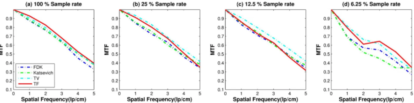
Image resolution—MTF. The Modulation Transfer Function (MTF) [43,44] is calculated to measure resolution of the reconstructed images. An Edge Spread Function (ESF) was obtained along the profile of the red line onFig 1. The Line Spread Function (LSF) was achieved by differentiating the ESF. The MTF was obtained from the Fourier transformation of the LSF. Normalization was performed as MTF(0) = 1.

Results

Evaluations with low-dose data

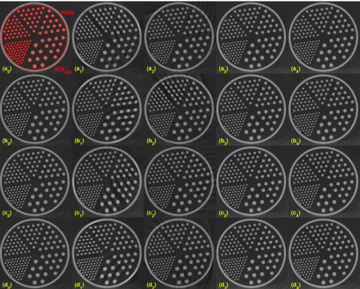
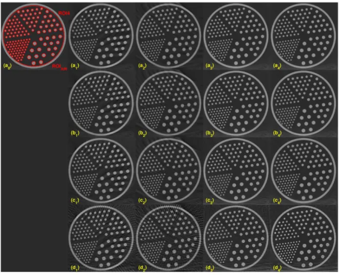
Four evaluations metrics were compared on the different dosage levels of 80, 100, 120, and 140 kVs. A different x-ray source has a different effective dosage (seeTable 1). We chose two slices for the evaluation process, slices 10 and 50. Figs1and2show the results for slices 10 and 50, respectively. For both figures, from left to right, each column shows the reconstructed images from the scanner, by FDK, Katsevich, TV, and TF algorithms. Each row consists of recon-structed images from different kVs: (aj)’s are from 80kV, (bj)’s are from 100 kV, (cj)’s are from

120 kV, and (dj)’s are from 140 kV, for allj = 0, � � �, 4. The red circles onFig 1indicate specific

ROIs; ROI1, ROI2, ROI3, and ROIAIRfor the computation of SNR and CNR. ROI 1, ROI2,

and ROI3 are the interior of the small circles inside the ACR phantom. The red line in (a0) is

the ROI for the edge spread function, used for calculating MTF. The set of interiors of the small red circles on the 50-th slice, the (a0) ofFig 2, is set as a ROI4 and the rest of the area

except ROI4 inside of the phantom is set to the ROIAIRfor the computation of the SNR and

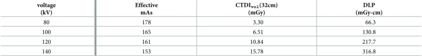
Table 1. Scan parameters with different voltages. voltage (kV) Effective mAs CTDIvol(32cm) (mGy) DLP (mGy-cm) 80 178 3.30 66.3 100 165 6.51 130.8 120 161 10.84 217.7 140 153 15.78 316.8 https://doi.org/10.1371/journal.pone.0210410.t001

(7)

CNR of ROI4. As illustrated in the Figs1and2, the images from TV and TF reconstruction algorithms give clear images compared to FDK and Katsevich results.

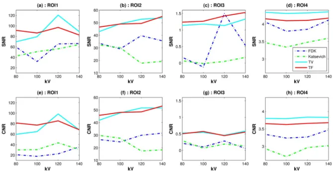
Quantitative evaluation results are shown in Figs3–5. For computing the UQI, images from the scanner were treated as true. Two ROIs for the UQI are set as the whole ACR phan-tom on the slices 10 and 50. The left bar plot ofFig 3shows the result of the UQI in three dif-ferent algorithms of the ROI on th 10th slice. The right plot shows the UQI result of slice 50. For both plots, the TF reconstruction method achieved the closest value to 1, which means the TF reconstructed image was the most similar to the scanner results. To evaluate the noise level of the reconstructed images,Fig 4shows the SNR and CNR results at the various dosage levels. The plots on the top row((a)-(d)) are the results of SNR over the ROI1, ROI2, ROI3, and ROI4. Note that each ROI has different y-range, since different ROI has different noise level. ROIs are defined in Figs1and2. CNRs on the ROI1-ROI4 are illustrated inFig 4(e)–4(h). TF and TV algorithms achieved the high CNR and SNR on the four ROIs at all dosage levels,

Fig 1. Illustrated reconstructed images with varying kVs on the slice number 10. (a0): Image from the scanner. Red circles indicate ROI’s: ROI1,

ROI2, ROI3 and ROIAIR. The red line is used to compute the LSF and MTF. Each row has reconstructed images at different kVs, (aj): 80kV, (bj): 100kV, (cj): 120kV, and (dj): 140 kV, for allj = 0 � � � 4. Each column has reconstructed images from different reconstruction algorithms: (X0): scanner, (X1):

FDK, (X2): Katsevich, (X3): TV, and (X4): TF for all letters X = a, b, c or d.

(8)

except in one case: The SNR on ROI3 at 120 kV. TF and TV algorithms are comparable. TF achieved the highest value on ROI3, but TV did on ROI4.

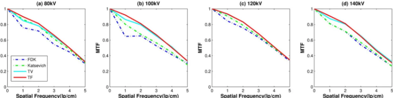
Fig 5shows the MTF curves of the results reconstructed by FDK, Katsevich, TV and the TF algorithm. Over all voltage levels, TF algorithms got the best resolutions than the other algo-rithms. But the MTF curve gives no big difference in various voltage levels.

Overall, quantitative evaluation results with various dosage show results of TF and TV are competitive.

Evaluations with sparse-view data

To evaluate with sparse-view performance, we fixed the dose level at 100kV. Images were reconstructed at four different sampling steps, 1, 4, 8, and 16. The full view data has 2304 views per 360˚. Sampling step 4 was achieved by taking 576 data uniformly per 360˚. Similarly, sam-pling steps 8 and 16 were achieved with 288 and 144 views per 360˚, respectively. For samsam-pling

Fig 2. Comparison of the reconstruction algorithms with varying kVs on the 50-th slice. ROI4 is the set of the interiors of the small red circles. ROIAIRis defined as the air part inside the phantom on slice 50-th. Each row has reconstructed images at different kVs, (aj): 80kV, (bj): 100kV, (cj): 120kV, and (dj): 140 kV, for allj = 0 � � � 4. Each column has reconstructed images from different reconstruction algorithms: (X0): scanner, (X1): FDK,

(X2): Katsevich, (X3): TV, and (X4): TF for all letters X = a, b, c or d.

(9)

step 4, it is equivalent that both the rotation speed and the table movement are four times faster than those of sampling step 1. The results of the reconstruction images with different view-angles are shown in Figs6and7. The images (a0) and (b0) are from the scanner on both

fig-ures. From the top to the bottom rows, images are reconstructed CT images by sampling steps 1, 4, 8, and 16. Each column shows images from a different reconstruction algorithm. From left to right, each column consists of images by scanner, FDK, Katsevich, TV and the TF

Fig 3. Image similarity measure: Bar plot of the UQIs of the different reconstruction algorithms over various dosage levels. (a): UQI on the 10-th slice, (b): UQI on the 50-th slice.

https://doi.org/10.1371/journal.pone.0210410.g003

Fig 4. Image noise measures: Plots of SNRs(top row) and CNRs(bottom row) with the different reconstruction algorithms over various voltage levels. Thex-axis is the dosage level in kV.

(10)

algorithm. As shown in the first row, reconstruction images at sampling step 1 are streak-free for all reconstruction algorithms. However, streaks appeared on the images with FDK and Kat-sevich for sparse-view data. The last column of the Figs6and7showed that visually TV and TF reconstruction outperformed other two reconstruction methods. On Figs6(a0)and7(a0),

Fig 5. Image resolution measure: Results of MTF curves with the different reconstruction algorithms over various voltage levels. The red line on theFig 1(a0)is used to compute LSF and MTF.

Fig 6. Reconstucted images with various sampling step sizes. From top to bottom, the sampling step size is set to 1, 4, 8, and 16. Each column consists of a different reconstruction algorithm, from left to right, scanner: FDK, Katsevich, TV and the TF algorithm. The image on (a0) shows

the three ROIs, and the red line is set for the computation of LSF for MTF. ROIAIR, ROI of air, is defined to compute the CNR for ROI1-ROI3.

(11)

ROI’s are defined as in the previous section. Visual comparison between TV and TF is given in the next subsection.

For the quantitative evaluation of similarity between the reconstructed image and the scan-ner image, we computed the UQI for each slices 10 and 50. The ROI for the UQI is set as the whole phantom area on a given slice.Fig 8shows the result of UQI with various sampling step sizes. Both plots (a) and (b) show that the TF algorithm achieved the highest value except one case, which means that the image reconstructed using the TF algorithm was the most similar to the scanner image.

For the quantitative evaluation of the noise level of the reconstructed images, we computed the SNR and CNR on ROIs 1–4.Fig 9shows the SNR and CNR results. Similar toFig 4, each column inFig 9has different y-range. The first row consists of the SNR results for ROI1-ROI4. The second row is the result of the CNR of ROI1-ROI4. Both SNR and CNR indices have a similar pattern. The TF algorithm achieved the highest SNR and CNR except for a few points in ROI2 and ROI4. For the quantitative evaluation of the image resolution,Fig 10shows MTF curves as described in the previous subsection. The LSF is computed with the ROI indicated inFig 6(a0). TV and TF results achieve high resolution than other two algorithms. The TF

Fig 7. Reconstucted images with various sampling step sizes. From top to bottom, the sampling step size is set to be 1, 4, 8, and 16. Each column consists of a different reconstruction algorithm, from left to right: scanner, FDK, Katsevich, TV and the TF algorithm. The image on (a0) shows ROI4 and ROIAIR.

(12)

algorithm achieved the highest MTF, especially when the fewest sample generated the highest MTF difference among other reconstructed methods.

Comparison with TV

As shown in Figs1~7, image qualities of TF and TV are hard to compare. Each quantitative metric shows a slight superiority of TF. To show some good points of the proposed algorithm, we have tested Rando phantom data, which has more realistic and complicated structure than ACR phantom. Rando phantom is scanned and reconstructed with sparse-view as done in the previous subsection.Fig 11shows the results by TV(top rows) and TF(bottom rows)

Fig 8. Image similarity measure: UQI results for various sampling step size.x- axis is the sampling step size, 1, 4, 8, and 16. y- axis is set as the UQI index. (a): UQI bar plot for the 10-th slice. (b): UQI bar plot for the 50th slice.

Fig 9. Image noise measures: SNR and CNR results for the various sampling step sizes. First row: SNR result, second row: CNR results.

(13)

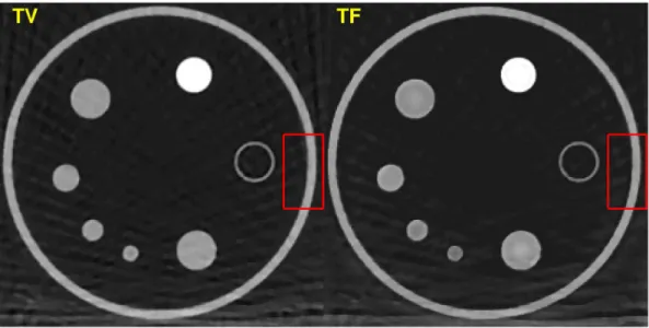
algorithms. The sampling size 1 (which is the right column) results shows similar to each other. But as the step size increases, the TV results are more blurry but clean, while that of TF maintains sharpen edges even with a large step size. Same results can be shown inFig 6.Fig 12 are same images fromFig 6, TV and TF reconstruction with step 16. Streaking artifacts due to partial projection data are shown less in the TF results. As indicated in red box, TF image has more sharpen edges than that of TV. Overall, we can conclude that TV and TF image qualities are similarly good, but TF has more sharpened edge and less artifacts.

One of the key factor to evaluate iterative algorithms is the reconstruction time. TV and TF elapsed times are summarized inTable 2. TF algorithm requires about 25% less time than TV algorithm.

Discussion and conclusion

To summarize, we have successfully developed a GPU-based TF iterative image reconstruction algorithm for low-dose multislice helical CT, and have shown that the TF method provided

Fig 10. Image resolution measure: Results of MTF curves with different reconstruction algorithms over various sampling levels. The red line on theFig 6(a0)is used to compute the LSF and MTF.

Fig 11. Visual quality comparison: TV(top row) and TF(bottom row). From left to right, reconstruction results by the sampling step size is set to 1, 4, 8, and 16. TV results shows more blurry effect compared to TF results.

(14)

improved image quality over the FDK, the Katsevich and TF algorithms when dealing with low-dose and sparse-view data, using UQI, SNR, CNR, and MTF measurements as evaluation metrics. High quality images are reconstructed by the proposed algorithm even with partial view data. TF algorithm is more computationally efficient than that of TV, because of the left-invertibility of the TF transform property [27]. Moreover, TV reconstructed images show more blurry and flattened than TF. The computational complexity of the TF algorithm is O(1), which is the cost of the x-ray transform and its adjoint per parallel thread [27].

Supporting information

S1 Fig. Data related toFig 1.

(MAT)

Table 2. TF and TV elapsed time in seconds.

sampling step size 1 4 8 16

TF 18199 4485 1708 718

TV 23303 5674 2692 1429

https://doi.org/10.1371/journal.pone.0210410.t002

Fig 12. Visual quality comparison: TV(left) and TF(right). TF image has less streaking artifact. As shown in the red box, TF maintain sharpen edge.

(15)

Author Contributions

Conceptualization: Haewon Nam, Lei Xing, Hao Gao.

Data curation: Haewon Nam, Keumsil Lee, Ruijiang Li, Bin Han. Formal analysis: Haewon Nam.

Funding acquisition: Rena Lee. Methodology: Haewon Nam, Hao Gao. Resources: Minghao Guo, Bin Han.

Software: Haewon Nam, Minghao Guo, Hengyong Yu, Keumsil Lee, Ruijiang Li. Supervision: Hengyong Yu, Lei Xing, Hao Gao.

Validation: Haewon Nam. Visualization: Haewon Nam.

Writing – original draft: Haewon Nam.

Writing – review & editing: Haewon Nam, Rena Lee, Hao Gao.

References

1. Hounsfield G. A method of apparatus for examination of a body by radiation such as x-ray or gamma radiation. US. Patent No. 1283925. 1972.

2. Mori I. Computerized tomographic apparatus utilizing a radiation source. US Patent No. 4630202. 1986. 3. Kalender WA, Seissler W, Klotz E, Vock P. Spiral volumetric CT with single-breathhold technique,

con-tinuous transport, and concon-tinuous scanner rotation. Radiol. 1990; 176(1): 181–183.https://doi.org/10. 1148/radiology.176.1.2353088

4. Feldkamp LA, Davis LC, Kress JW. Practical cone-beam algorithm. JOSA A. 1984; 1(6): 612–619. https://doi.org/10.1364/JOSAA.1.000612

5. Wang G, Lin TH, Cheng PC, Shinozaki DM. A general cone-beam reconstruction algorithm. Med. Img. IEEE Trans. 1993; 12(3): 486–496.https://doi.org/10.1109/42.241876

6. Hein I, Taguchi K, Silver M, Kazarna M, Mori I. Feldkamp-based cone-beam reconstruction for gantry-tilted helical multislice CT, Med. Phys.2003; 12: 3233–3242.https://doi.org/10.1118/1.1625443 7. Zhao J, Lu Y, Jin Y, Bai E, Wang G. Feldkamp-type reconstruction algorithms for spiral cone-beam CT

with variable pitch. J. of X-Ray Sci. and Tech. 2007; 15: 177–196.

8. Taguchi K, Aradate H. Algorithm for image reconstruction in multi-slice helical CT. Med. Phys. 1998; 25: 550–561.https://doi.org/10.1118/1.598230PMID:9571623

9. Katsevich A. Theoretically exact filtered backprojection-type inversion algorithm for spiral CT. SIAM J. Appl. Math. 2002; 62: 2012–2026.https://doi.org/10.1137/S0036139901387186

10. Katsevich A. Analysis of an exact inversion algorithm for spiral cone-beam CT. Phys. Med. Biol. 2002; 47: 2583–2597.https://doi.org/10.1088/0031-9155/47/15/302PMID:12200926

11. Katsevich A. An improved exact filtered backprojection algorithm for spiral computed tomography. Adv. Appl. Math. 2004; 32: 681–697.https://doi.org/10.1016/S0196-8858(03)00099-X

12. Noo F, Pack J, Heuscher D. Exact helical reconstruction using native cone-beam geometries. Phys. Med. Biol. 2003; 48: 3787–3818.https://doi.org/10.1088/0031-9155/48/23/001PMID:14703159 13. Yu H, Wang G. Studies on implementation of the Katsevich algorithm for spiral cone-beam CT. J.

X-Ray Sci. Technol. 2004; 12: 97–116.

14. Chen GH. An alternative derivation of Katsevich’s cone-beam reconstruction formula. Med. phys. 2003; 30(12): 3217–3226.https://doi.org/10.1118/1.1628413PMID:14713088

15. Zou Y, and Pan X. Exact image reconstruction on Pi-linew from minimum data in helical cone-beam CT. Phys. Med. Biol. 2004; 49: 941–959.

16. Zou Y, Pan X. Image reconstruction on PI-lines by use of filtered backprojection in helical cone-beam CT. Phys, in Med. and Bio. 2004; 49(12): 2717.https://doi.org/10.1088/0031-9155/49/12/017

(16)

17. Ye Y, Wang G. Filtered backprojection formula for exact image reconstruction from cone-beam data along a general scanning curve. Med. Phys. 2005: 32(1); 42–48.https://doi.org/10.1118/1.1828673 PMID:15719953

18. Ye Y, Zhao S, Yu H, Wang G. A general exact reconstruction for cone-beam CT via backprojection-fil-tration. Med Img IEEE Trans. 2005; 24(9): 1190–1198.https://doi.org/10.1109/TMI.2005.853626 19. Cho S, Xia D, Pelizzari CA, Pan X. Exact reconstruction of volumetric images in reverse helical

cone-beam CT. Med. Phys. 2008; 35(7): 3030–3040.https://doi.org/10.1118/1.2936219PMID:18697525 20. Ye Y, Yu H, and Wang G. Gel’fand–Graev’s reconstruction formula in the 3D real space. Med. Phys.

2011; 38(S1): S69–S75.https://doi.org/10.1118/1.3577765PMID:21978119

21. Thibault JB, Sauer KD, Bouman CA, Hsieh J. A three-dimensional statistical approach to improved image quality for multislice helical CT. Med. Phys. 2007; 34(11): 4526–4544.https://doi.org/10.1118/1. 2789499PMID:18072519

22. Nuyts J, Man BD, Dupont P, Defrise M, Suetens P, Mortelmans L. Iterative reconstruction for helical CT: a simulation study. Phys. Med. Biol. 1998; 43: 729–737.https://doi.org/10.1088/0031-9155/43/4/ 003PMID:9572499

23. Gordon R, Bender R, Herman GT. Algebraic reconstruction techniques (ART) for three-dimensional electron microscopy and X-ray photography. J. of Theo. Bio. 1970; 29(3): 471–481.https://doi.org/10. 1016/0022-5193(70)90109-8

24. Anderson AH, Kak AC. Simultaneous algebraic reconstruction technique (sART): A superior implemen-tation of the art algorithm. Ultrasonic Imaging. 1984; 6: 81–94.https://doi.org/10.1016/0161-7346(84) 90008-7

25. Sunnegårdh J, Grasruck M. Nonlinear regularization of iterative weighted filtered backprojection for heli-cal cone-beam CT. IEEE Nuclear Sci. Symposium. 2008; 43: 5090–5095.

26. Yu W, Zeng L. Iterative image reconstruction for limited-angle inverse helical cone-beam computed tomography. Scanning. 2016; 38(1): 4–13.https://doi.org/10.1002/sca.21235PMID:26130367 27. Gao H, Li T, Lin Y, Xing L. 4D cone beam CT via spatiotemporal tensor framelet. Med. Phys. Letter.

2012; 39: 6943–6946.

28. Gao H, Qi XS, Gao Y, Low DA. Megavoltage CT imaging quality improvement on TomoTherapy via ten-sor framelet. Med. Phys. 2013; 40(8): 081919.https://doi.org/10.1118/1.4816303PMID:23927333 29. Donoho DL. Compressed sensing. IEEE Transactions on Info. Theory. 2006; 52(4): 1289–1306.

https://doi.org/10.1109/TIT.2006.871582

30. Candès EF, Romberg J, Tao T. Robust uncertainty principles: Exact signal reconstruction from highly incomplete frequency information. IEEE Transactions on Information Theory. 2006; 52(2): 489–509. https://doi.org/10.1109/TIT.2005.862083

31. Sidky EY, Kao CM, Pan X. Accurate image reconstruction from few-views and limited-angle data in divergent-beam CT. J. X-Ray Sci. Tech. 2006; 14: 119–139.

32. Chen GH, Tang J, Leng S. Prior image constrained compressed sensing (PICCS): a method to accu-rately reconstruct dynamic CT images from highly undersampled projection data sets. Med. Phys. 2008; 35(2): 660–663.https://doi.org/10.1118/1.2836423PMID:18383687

33. Yu H, Wang G. Compressed sensing based interior tomography. Phys. Med. Bio. 2009; 54(9): 2791. https://doi.org/10.1088/0031-9155/54/9/014

34. Gao H, Cai JF, Shen Z, Zhao H. Robust principal component analysis based four dimensional com-puted tomography. Phys. Med. Biol. 2011; 56: 3181–3198.https://doi.org/10.1088/0031-9155/56/11/ 002PMID:21540490

35. Gao H, Yu H, Osher S, Wang G. Multi-energy CT based on a prior rank, intensity and sparsity model (PRISM). Inverse Probl. 2011; 27: 115012.https://doi.org/10.1088/0266-5611/27/11/115012PMID: 22223929

36. Jia X, Dong B, Lou Y, Jiang SB. GPU-based iterative cone-beam CT reconstruction using tight frame regularization. Phy. Med. Biol. 2011; 56(13); 3787.https://doi.org/10.1088/0031-9155/56/13/004 37. Xu Q, Yu H, Mou X, Zhang L, Hsieh J, Wang G. Low-dose X-ray CT reconstruction via dictionary

learn-ing. IEEE Trans. Med. Img. 2012; 31(9): 1682–1697.https://doi.org/10.1109/TMI.2012.2195669 38. Flohr TG, Stierstorfer K, Ulzheimer S, Bruder H, Primak AN, McCollough CH. Image reconstruction and

image quality evaluation for a 64-slice CT scanner with z-flying focal spot. Med Phys. 2005; 32(8): 2536–2547.https://doi.org/10.1118/1.1949787PMID:16193784

39. Gao H. Fast parallel algorithms for the x-ray transform and its adjoint. Med Phys. 2012; 39(11): 7110– 7120.https://doi.org/10.1118/1.4761867PMID:23127102

40. Dong B, Shen Z. MRA based wavelet frames and applications. IAS Lecture Notes Series, Summer Pro-gram on “The Mathematics of Image Processing”, Park City Mathematics Institute. 2010; 19.

(17)

41. Boyd S, Parikh N, Chu E, Peleato B, Eckstein J. Distributed optimization and statistical learning via the alternating direction method of multipliers, Foundations and Trends®in Machine Learning. 2011; 3(1): 1–122.

42. Goldstein T, Osher S. The Split Bregman method for L1-regularized problems. SIAM J. Imaging Sci. 2009; 2: 323–373.https://doi.org/10.1137/080725891

43. Gao Y, Bian Z, Huang J, Zhang Y, Niu S, Feng Q et al. Low-dose X-ray computed tomography image reconstruction with a combined low-mAs and sparse-view protocol. Optics Exp. 2014; 22(12): 15190– 15210.https://doi.org/10.1364/OE.22.015190

44. Judy PF. The line spread function and modulation transfer function of a computed tomographic scanner. Med Phys. 1976; 3(4): 233–236.https://doi.org/10.1118/1.594283PMID:785200