1. INTRODUCTION
Today, high speed aircrafts like military aircrafts are demanded to perform various maneuvers and missions with high risk in battle field. According to this demand, many researches concerning about nonlinear flight dynamics have been attracted in the field of flight control system design, which are those away from the conventional approaches of flight control system designs based on aircraft linear flight dynamics. However, the linear flight control systems, designed in linear control theories such as classical control, optimal control like LQG/LTR and several robust controls of
theory and −
∞ H
H /2 µ synthesis and many others, are − still valuable and popular in aircraft industry. These techniques have a common procedure in the flight control system design: first of all, nonlinear flight dynamics of the associated aircraft are linearized around important trim points located within the overall flight envelope, and then apply linear control theories to each of the linear models to satisfy the handling qualities given in several MIL specs like MIL-8785C. Once appropriate flight control laws at each of trim points are designed, finally, gain scheduling is applied to those of the flight control systems to complete the final control system design. Usually gain scheduling is in charge of variation of control laws to airspeed, angle of attack and dynamic pressure. Also this approach can cover, to a certain extent, robustness to uncertainties of aerodynamics and nonlinearities of aircraft dynamics due to linear model-based design. However, this approach needs a lot of time and effort to get to a final design. Hence, in this paper, we propose an adaptive nonlinear control technique to design a robust flight control system efficiently. This technique is based on linear control and adaptive neural network so there is no need of gain scheduling. In this flight control proposed, the linear control structure consists of Stability Augmentation and Hold Autopilot, and the adaptive neural network has a role of canceling uncertainties of aerodynamics and variation of flight dynamics due to change of trim points.
Among various kinds of flight maneuvers, approach landing is the most dangerous since airspeed of this maneuver is very low near stall region and angle of attack is very high near maximum lift. Also pilot work load is extremely high in this fight region. Because of this situation, domestic aircraft accident record showed that the pilot’s mistake is one of the main reasons of the accidents. Moreover more than 50% among accidents occur in the approach and landing maneuver. Hence, auto-landing is most preferable to reduce accidents originated from pilot’s mistake due heavy pilot workload. In
this paper, we will design an auto-landing guidance and control system in adaptive nonlinear control technique proposed in this study, which is based on linear controller combined with neural network. In this approach, first of all, an auto-landing linear tracking controller satisfying the handling quality is designed in classical design technique. In the next the adaptive neural network with single hidden layer is introduced to compensate for model error between the reference tracking model and the outputs of the feedback control system coming out of the nonlinear aircraft model. To satisfy the overall closed-loop stability, Lyapunov stability concept is applied to the closed-loop system based on the linear feedback controller and the adaptive neural network. From this result, a set of on-line weight update rules for the neural network, whose activation function is sigmoidal function, will be obtained. This proposed design technique for longitudinal auto-landing maneuver is evaluated in the nonlinear aircraft simulation model: initial flight conditions are 1500 ft altitude and 250 ft/se velocity in level flight and the associated aircraft is about to the approach landing. In section 2, overall picture of linear controller-based neural network compensation technique is briefly explained, and the multiplayer neural network to be used in this paper is discussed in details in section 3. In section 4, this technique is applied to auto-landing guidance and control system design, and conclusion is followed in section 5.
Design of Longitudinal Auto-landing Guidance and Control System
Using Linear Controller-based Adaptive Neural Network
Si-Young Choi*, Cheolkeun Ha
** Department of Aerospace Engineering, University of Ulsan, Korea (Tel : +82-52-259-2590; E-mail: [email protected])
Abstract: We proposed a design technique for auto-landing guidance and control system. This technique utilizes linear controller and neural network. Main features of this technique is to use conventional linear controller and compensate for the error coming from the model uncertainties and/or reference model mismatch. In this study, the multi-perceptron neural network with single hidden layer is adopted to compensate for the errors. Glide-slope capture logic for auto-landing guidance and control system is designed in this technique. From the simulation results, it is observed that the responses of velocity and pitch angle to commands are fairly good, which are directly related to control inputs of throttle and elevator, respectively.
Keywords: Linear Controller, Neural Network, Lyapunov Stability, Glide-slope Capture Logic
2. SYSTEM DESCRIPTIONS
In general a nonlinear system is described in the following form of Eq.(1), ]) , [ (u xu B Ax x&= + +∆ (1) where state vector
x
∈
R
n, control input vector m, andR
u
∈
], [xu
∆ denotes approximate error or uncertainty in nonlinear system. In this paper, it is assumed that we already have a linear controller for inner-loop (stability) and outer-loop (command) of the overall structure of control system. This structure is shown in Fig.1. Note that the associated matrices in Fig.1 implies inner-loop controller of the matrices with subscript (η) and the outer-loop controller of the matrices with subscript(ρ ).
ICCAS2005 June 2-5, KINTEX, Gyeonggi-Do, Korea
ICCAS2005 June 2-5, KINTEX, Gyeonggi-Do, Korea
η A Bη η C Dη A B C D ρ A Bρ ρ C Dρ
+
− + − ϑy
ρ y ηy
ρu
ηu
u
Figure 1. Linear Control System Designed
The closed-loop state equation of this control structure is expressed in Eq.(2) and Eq.(3).
] , [ * * B y B xu A + + ∆ = ϑ ϑ ∆ ϑ& (2) ϑ ϑ C* y = (3) From the state equation in Eq.(2) and Eq.(3), a linear equation excluding the uncertain matrix term is obtained shown in Eq.(4). This is the reference model to which the nonlinear plant model should follow in the final feedback system.
ϑ ϑ ϑ&R=A* R+B*y (4) R R C y = *ϑ (5) where the input in Fig.1 is defined to be
η ρ u u
u= −
(6) Now define the error state to be the error between the state coming from Eq.(4) and the state coming from the plant model in Eq.(1). The error state equation is obtained in Eq.(8).
ϑ ϑ − = R e (7) ] , [ *e B xu A e&= − ∆∆
(8)
Since the approximate error or uncertainty in nonlinear plant exist in the term of , canceling those effects is required in the overall closed-loop system. In this study, we introduce neural network to this approach. The neural network input is added to the control input in Eq.(6), and then the total control input is defined as in Eq.(9).
] , [ ux ∆ ad u u u u= ρ− η−ˆ (9) Therefore the error dynamical equation is expressed again in Eq.(10). ]) , [ ˆ ( *e B u xu A e&= − ∆ ad−∆ (10) where
A
*andB
∆are defined in Eq.(2), respectively.3. MULTILAYER NEURAL NETWORKS
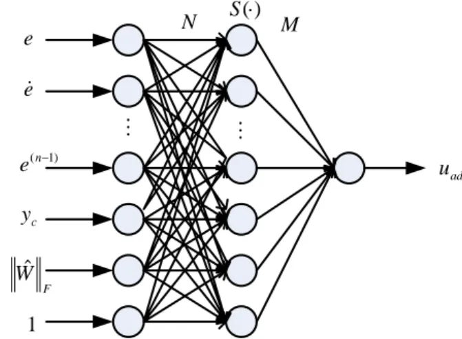
In this paper, we introduce a neural network with single hidden layer, which is defined in Eq.(11).) ( )
(z M S N z
g = T T (11) where the coefficient matrix between output layer and hidden layer denotes MT∈Rl
,
and the coefficient matrix between input layer and hidden layer.
Also the input variables into neural network is selected to bel n T R N ∈ ( +3)* 3 1 ˆ ∈ + ⎥⎦ ⎤ ⎢⎣ ⎡ = n F T R W y e z ϑ
.
Also is an activatefunction. In this study this function is Sigmoidal function defined to be ) (⋅ S a z a e z
S( )= 11 + − . When an ideal solution of the weighting matrices of the neural network are M*an , respectively, the approximate of them are the matrices of
*
N Mˆ and , respectively. The error matrices between the ideal and approximate matrices are defined as
Nˆ * ˆ ~ M M M= − , * ˆ ~ N N
N= − . Note that the neural network with ideal coefficient matrices is given in Eq.(12),
ε + = ( ) ) ( * * * z M S N z uad T T (12) where
ε
means boundary layer due to finite number of neural network layer.e
e
&
) 1 (n−e
cy
FWˆ
1
adu
)
(⋅
S
N
M
M
M
Figure 2. Neural Network Structure with Single Hidden Layer Note that the error between the linear model and the nonlinear model is supposed to be approximated in the neural network. If the error and uncertainty , shown in Eq.(2), is ideally modeled, then the neural network is substituted into Eq.(10). After rewriting the expression, we obtained the following form in Eq.(13),
]
,
[ u
x
∆
) ~ ˆ ˆ ) ˆ ˆ ˆ ( ~ ( * r T T T T v w z N S M z N S S M B e A e&= − ∆ − ′ + ′ −ε+ + (13) where is the higher order terms of , which isexpressed to be
w
2 ) (⋅ Oz
N
S
M
z
N
O
M
w
=
*T(
~
T)
2+
~
Tˆ
*T (14) and denotes the term to cancel the error between the higher order term in Eq.(14) and the boundary layer (r
v
ε
). Also it is defined to be ) ˆ ( ˆ S N z S= T and Sˆ′=diag{sˆ1′,sˆ2′,Lsˆl′} (15) Note that si s niTz d[
s za dza]
z nTz i l i a , 1,2,L / ) ( ) ˆ ( ˆ′= ′ = =ˆ = .In order that the overall closed-loop system should be stable, the following Lyapunov function is introduced, as shown in Eq.(16),
ICCAS2005 June 2-5, KINTEX, Gyeonggi-Do, Korea
{
} {
T N T M T N N tr M M tr Pe e V ~ ~ 2 1 ~ ~ 2 1 2 1 + Π−1 + Π−1 =}
(16)where the positive definite symmetric matrix P is obtained from the algebraic Lyapunov equation in Eq.(17).
I PA P
A*T + *T =−2 (17) Here the update rule for the neural network are defined to be as follows,
(
)
[
S SN z M]
M&ˆ =−ΠM ˆ− ˆ′ˆT λ+σλ ˆ (18)[
z M S N N&ˆ=−ΠNλ
ˆTˆ′+σ
λ
ˆ]
(19) λ λ λ v F w r k W W e k v ⎟ + ⎠ ⎞ ⎜ ⎝ ⎛ + = ˆ (20) where the parameter (λ
) and the stacked weighting matrix (wˆ ) are defined to be ∆ = PBeT λ (21) ⎥ ⎥ ⎦ ⎤ ⎢ ⎢ ⎣ ⎡ = M N W ˆ 0 0 ˆ ˆ (22)Note that real values of and are positive, and w
k
kvF Wˆ is Frobenius norm of W. Also training rate of the neural network (
Π
,Π
) should be positive. Once we got those for Eq.(16), then the first derivative of the Lyapunov function should be negative in order that the overall closed-loop system is stable.ˆ
M N
Now, take a derivative in Eq.(16) and derive the derivative gain by substituting Eq.(13), Eq.(17), Eq.(18) and Eq.(19). a ) ˆ ( ) ~ ( ~ ) ( 2 2 2 W W k k W W W w e V W V − + − + + + + − ≤ λ λ λ σ ε λ & (23)
where w can be rewritten from Eq.(14) to be as
2 3 2 1 0 c Wˆ c Wˆ c Wˆ c w≤ + + λ + (24) Furthermore Eq.(23) becomes as follows,
λ λ2 1 0 2 a a e V&≤− − + (25) where 0 1 2 3 1 2 0 ~ ) ( ~ ) ( ~ ) ( 2 c W c W W c a W c k W k k a V W W + + + + − = − + + = ε σ σ (26)
Therefore becomes negative when the following terms are satisfied: , ,
V&
2
c
kW > a0>0 λ >a1/a0 .
4. APPLICATION TO GLIDESLOPE CAPTURE
LOGIC DESIGN FOR AUTOLANDING
PROBLEM
In this section, an auto-landing guidance and control system will be designed in the technique proposed in the previous sections. The design process for auto-landing control system is that first, an appropriate linear controller is designed, for an
example, in classical root-locus method. Then after formulating the problem in state space in which the proposed design technique needs, we design a proper neural network. In this study, a glide-slope capture logic in longitudinal motion is only considered to apply this proposed technique to auto-landing control system. The control logic designed consists of the inner-loop (velocity stabilization and stability augmentation) and the outer-loop (pitch command). Also the glide-slope capture logic as guidance logic is designed to simulate auto-landing situation. The trim at which the linear aircraft model is obtained is unstable so stability augmentation logic is required. Once the linear control system with good stability and command following performance is designed as the reference model, the overall closed-loop system in nonlinear aircraft model with the linear control system is composed. In order to evaluate performance of the overall system, two commands of velocity (250 ft/sec) and pitch angle are added to the nonlinear aircraft model, where the pitch angle command is generated by glide-slope capture guidance logic. In the numerical simulation, the associated aircraft starts landing maneuver at the trim of altitude 1500ft, airspeed 250 ft/sec and a level flight with flight path angle 3 deg.
The linear model of the associated aircraft is defined in Eq.(27) and Eq.(28).
U B X A X&= F + F (27) U D X C Y= F + F (28) where the state variables and the control inputs are
[
]
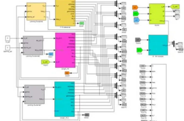
T e t t q P V X= α θ δ δ [ ]T e t u u U=and and denote throttle (%) and elevator (deg), respectively. Inputs to the neural network are state variables of the aircraft and norm of the weighting matrices and neural network outputs itself. The overall simulation block diagram in Matlab/Simulink is depicted in Fig.3.
t
u ue
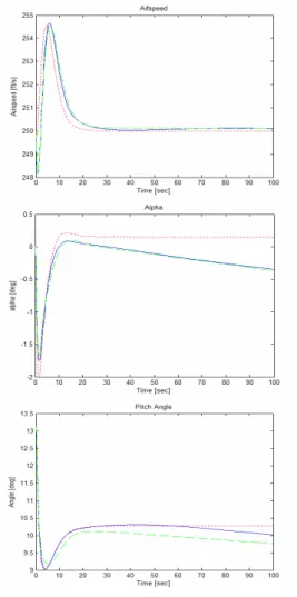
Figure 3. Overall Block Diagram in Matlab/Simulink In this design, design parameters for the neural network are determined to be as ΠM= 0.03, ΠN= 0.1, σ = 0.0005, = 0.004, =0.001. Since the control inputs are elevator and throttle, two commands are selected so that the commands of velocity and pitch angle will expect to show reasonable performance. In fig.4, the time responses of the glide-slope capture logic to the commands are shown and compared with each other. The response shown in dotted line is that coming from the reference model, and the response in the solid line is that which is compensated in the neural network for the error
w
k
v
k
ICCAS2005 June 2-5, KINTEX, Gyeonggi-Do, Korea
between the reference model and the nonlinear plant. From the figure in Fig.4, the responses of velocity and pitch angle are fairly good to follow the commands of velocity and pitch angle during the glide-slope capture. The other responses show reasonable results but do not have accurate model following characteristics: angle of attack and flight path angle. This problem comes from insufficient control inputs in the nonlinear plant. However effect of neural network on compensation for the error existing during the glide-slope capture maneuver can be seen in Fig.5. The 2 norm of the error is shown where the dotted line shows uncompensated responses and the solid line implies compensated response to the commands. The altitude response, however, is fairly acceptable even though some error between reference and real response exits.
5. CONCLUSIONS
So far we proposed a design technique for auto-landing guidance and control system. Main features of this design technique is to use conventional linear controller and compensate for the error coming from the model uncertainties and/or reference model mismatch. In this study, the multi-perceptron neural network with single hidden layer is adopted to compensate for the errors. From the simulation results, it is observed that the responses of velocity and pitch angle to commands are fairly good, which are directly related to control inputs of throttle and elevator, respectively.
Figure 4. Time Responses to Commands
Figure 5. 2 Norm of the Error Between Ref. Model and Nonlinear Plant Model
REFERENCES
[1] Manu Sharma and Anthony J. Calise, “Neural Network Of Augmentation of Existing Linear Controllers,” AIAA Guidance, Navigation, and Control Conference. AIAA 2001-4163, August 2001.
[2] Seungjea Lee, “Neural Network Based Adaptive Control and Its Applications to Aerial Vehicles,” Georgia Institute of Technology, April, 2001.
[3] Brian L.Stevens and Frank L. Lewis, “Aircraft Control and Simulation,” Wiley Interscience, 1992