y (t) R (t)
1. INTRODUCTION
The best-known controllers used in industrial control processes are proportional-integral-derivative (PID) controllers because of their simple structure and robust performance in a wide range of operating conditions. The design of such a controller requires specification of three parameters: proportional gain, integral time constant and derivative time constant .so far, great effort has been devoted to develop methods to reduce the time spent on optimizing the choice of controller parameters [1].
Setting the PID parameters are called tuning ,the classical tuning method is to use the famous Ziegler-Nichols tuning formula. This tuning formula however, is not always effective in the sense that it may completely fail to tune the processes with, for example, relatively large dead time.
Moreover, its tuning will have to be supplemented with purely experience-based fine-tuning to meet the specifications [2].
The parameters of the PID controller kp, ki and kd (or kp, Ti and Td) can be manipulated to produce various response curves from a given process as we will see later.
2. PID CONTROLLER
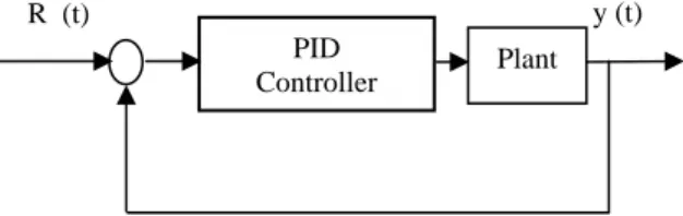
PID controllers are commonly used to regulate the time-domain behavior of many different types of dynamic plants. These controllers are extremely popular because they can usually provide good closed-loop response characteristics, can be tuned using relatively simple design rules, and are easy to construct using either analog or digital components. Consider the feedback system architecture that is shown in Fig. 1 where it can be assumed that the plant is a DC motor whose speed must be accurately regulated.
Fig. 1 Feedback system architecture
The PID controller is placed in the forward path, so that its output becomes the voltage applied to the motor's armature .the feedback signal is a velocity, measured by a tachometer .the output velocity signal y (t) is summed with a reference or command signal R (t) to form the error signal e (t). Finally, the
error signal is the input to the PID controller.
Before examining the input-output relationships and design methods for the PID controller, it is helpful to review typical characteristics observed for the velocity response of a DC motor to a step voltage input. Different characteristics of the motor response (steady-state error, peak overshoot, rise time, settling time, etc) are controlled by selection of the three gains that modify the PID controller dynamiclly.
This is discussed in detail below .the PID controller is defined by the following relationship between the controller input e (t) and the controller output u (t) that is applied to the motor armature:
∫
×
+
×
×
+
×
=
tdt
t
de
kd
d
e
ki
t
e
kp
t
u
0)
(
)
(
)
(
)
(
τ
τ
(1)Taking the Laplace transform of this equation gives the transfer function G(s):
)
(
)
(
)
(
)
(
kd
s
s
ki
kp
t
e
t
u
s
G
=
=
+
+
×
(2) This transfer function clearly illustrates the proportional, integral and derivative gains that make up the PID compensation. Select new definitions for the gain terms according to:kp
=
k
.
Ti
k
ki
=
kd
=
k
×
Td
)
(
)
(
k
Td
s
s
Ti
k
k
s
G
+
×
×
×
+
=
(
)
(
1
1
Td
s
)
s
Ti
k
s
G
+
×
×
+
=
)
1
1
(
)
(
Td
s
s
Ti
kp
s
G
+
×
×
+
=
(3) The discrete-time equation expression is given as:)
(
)
(
)
(
)
(
1k
e
kd
i
e
ki
k
e
kp
k
u
T
T
s n i s+
∆
×
+
×
=
∑
= (4)DC MOTOR SPEED CONTROL USING PID CONTROLLER
Fatiha Loucif
Department of Electrical Engineering and information, Hunan University, ChangSha, Hunan, China (E-mail:[email protected])
Abstract. The PID controller design and choosing PID parameters according to system response are proposed in this paper. Here
PID controller is employed to control DC motor speed and Matlab program is used for calculation and simulation. Choosing PID parameters are demonstrated by several contrast experiments and a way for setting PID parameters values is discussed.
Keywords: PID controller, DC motor, Matlab representation, P control, PI control, PID control.
PID
Here, u (k) is the control signal, e (k) is the error, Ts is the sampling period for the controller, and
)
1
(
)
(
)
(
≈
−
−
∆
e
k
e
k
e
k
2.1 Physical setup and system equation:
DC motors have speed-control capability, which means that speed, torque and even direction of rotation can be changed at any time to meet new conditions [3] .The electric circuit of the armature and the free body diagram of the rotor are shown in the following figure:
Fig. 2 electric circuit and free body diagram
For this example, we will assume the following values for the physical parameters.
Moment of inertia of the rotor (J) =0.01 kg.m^2/s^2. Damping ratio of the mechanical system (b)= 0.1 nms. Electromotive force constant (k=ke=kt)=0.01 nm/amp. Electric resistance (R) =1 ohm.
Electric inductance (L)= 0.5 H. Input (v): source voltage. Output (theta): position of shaft.
The rotor and shaft are assumed to be rigid.
The motor torque T, is related to the armature current i, by a constant factor kt. The back emf, is related to the rotational velocity by the following equations:
i
kt
T
=
×
.e
=
emf
=
ke
×
θ
&
.In SI units (which we will use),kt (armature constant) is equal to ke (motor constant) .
From the figure above we can write the following equations based on Newton’s law combined with kirchhoff`s law:
i
k
b
J
×
θ
&&
+
×
θ
&
=
×
..
θ
&
×
−
=
×
+
×
R
i
V
k
dt
di
L
2.2 Transfer function:
Using Laplace transforms, the above modeling equations can be expressed in terms of s.
S
(
J
×
s
+
b
)
×
θ
(
s
)
=
k
×
i
(
s
).
(
L
×
s
+
R
)
×
i
(
s
)
=
V
−
k
×
s
×
θ
(
s
).
by eliminating i(s) we can get the following open-loop transfer function ,where the rotational speed is the output and the voltage is the input .
k
R
s
L
b
s
J
k
V
2)
(
)
(
×
+
×
×
+
+
=
θ
.3. DESIGN REQUIREMENTS:
First, our uncompensated motor can only rotate at 0.1 rad/sec with an input voltage of 1 volt (this will be demonstrated later when the open-loop response is simulated. since the most basic requirement of a motor is that it should rotate
At the desired speed, the steady-state error of the motor speed should be less than 1% .the other performance requirement is that the motor must accelerate to its steady-state speed as soon as it turn on. In this case, we want it to have a settling time of less than 2 seconds. Since a speed faster than the reference may damage the equipment, we want to have an overshoot of less than 5%.
If we simulate the reference input(R) by a unit step input, then the motor speed output should have:
Settling time less than 2seconds. Overshoot less than 5%. Steady-state error less than 1%.
4- MATLAB REPRESENTATION AND
SYSTEM RESPONSE:
4.1. Open-loop response:
4.1.1. Transfer function: we can represent the above transfer
function into Matlab by the numerator and denominator matrices as follows
num =k
den :=(J*s +b)*(L*s+R) +k^ 2 *The m-file is as follow (program 1): J=0.01; b=0.1; k=0.01; R=1; L=0. 5; num=k; den=[(J*L) ((J*R)+(L*b)) ((b*R) + k^2)]; Step (num, den, 0:0.1:3)
Fig. 3 open loop response.
From the plot we see that when 1 volt applied to the system, the motor can only achieve a maximum speed of 0.1 rad/sec, ten times smaller than our desired speed. Also, it takes the motor 3 seconds to reach its steady-state speed; this does not satisfy our 2 seconds settling time criterion.
4.2. Closed-loop response:
The closed-loop program looks like (program 2): J=0. 01; b=0.1; k=0.01; R=1; L=0. 5; num=k; den=[ (J*L) ((J*R)+(L*b)) ((b*R) + k^2)] ;
%%%%% Different values of kp , ki and kd %%%%%%%%% kp= ; ki= ; kd= ; numc=[kd,kp,ki]; denc=[0 1]; numa=conv(num,numc); dena=conv(den,denc); [numac,denac]=cloop(numa,dena); step(numac,denac) xlabel('time(sec)'), ylabel('velocity(rad/sec)') Title (`pid control `)
Grid;
5- PROPORTIONAL CONTROL:
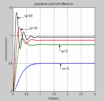
Let's first try using a proportional controller; so we set ki=0, kd=0 in program (2) And we take different values of kp the
calculation results was assumed in Table 1, and the corresponding plots was gathered in Fig. 4:
Table 1 kp Rise time(sec) Maximum overshoot (%) Steady State error Peak amplitude 10 0.488 / 0.5 0.5 0 0.301 / 0.334 0.681 50 0.158 / 0.167 0.94 70 0.125 4 0.125 1.04 100 0.097 14 0.091 1.14 200 0.064 32 0.048 1.32 300 0.051 41 0.032 1.41
We see that the proportional controller kp have the effect of reducing the rise time; from (0.48sec) for kp=10 to (0.051sec) for kp=300; and will reduce and never eliminate the steady-state error from (0.5) for kp=10 to (0.032) for kp=300. so the response becomes more and more faster by increasing the gain kp. But will increase the maximum overshoot; from (4% to 41%).
Fig. 4 closed loop response with different values of kp .
6- PROPORTIONAL INTEGRAL CONTROL
(PI):
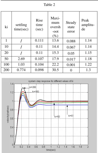
The settling is time still too long, we try now to increase the gain ki with kp=100, all the results are shown in the Table 2. And the corresponding plot is gathered in Fig. 5.
Table 2 ki settling time(sec) Rise time (sec) Maxi-mum oversh -oot (%) Steady state error Peak amplitu-de 1
/
0.111 13.6 0.088 1.14 10/
0.11 14.4 0.067 1.14 20/
0.11 15.3 0.05 1.15 50 2.69 0.107 17.9 0.017 1.18 100 1.03 0.104 22.2 0.001 1.22 200 0.774 0.098 30.5 0 1.3Fig. 5 closed loop response with different values of ki. Now we see that the response is much faster than before; the settling time becomes (0.774 sec) for ki=200, and the steady-state error becomes very small and eliminated for ki=200.
7-PROPORTIONAL-INTEGRAL-DERIVATIV
E CONTROL (PID):
Now, we increase the gain kd, with kp=100;ki=200. All results are illustrated in the Table 3 and the corresponding plots are shown in Fig. 6.
From the results we see that the settling time reduced from (0.58 sec to 0.257sec) for (kd=1 to kd=10) and the overshoot from (23% to 1.03%) and there is small change in the rise time. Table 3 kd settling time(sec) Rise time (sec) Maxi-mum oversh oot(%) Steady state error Peak amplitude 1 0.588 0.106 23 0 1.23 3 0.403 0.116 12.6 0 1.13 5 0.419 0.121 6.09 0 1.06 8 0.201 0.127 1.43 0 1.01 10 0.257 0.132 1.03 0 1.01
Fig. 6 closed loop response with different values of kd. So now we know that if we use a pid controller with: kp=100,ki=200 and kd=10; all our design requirements will be satisfied and the response looks like:
Fig. 7 system closed loop response with PID control.
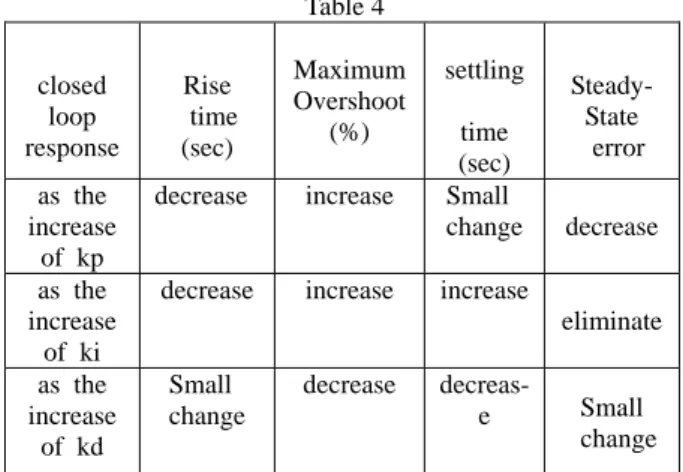
Effects of PID controllers parameters kp, ki and kd on a closed loop system are summarized in the table bellow.
Table 4 closed loop response Rise time (sec) Maximum Overshoot (%) settling time (sec) Steady- State error as the increase of kp
decrease increase Small
change decrease as the
increase of ki
decrease increase increase eliminate as the increase of kd Small change decrease decreas-e Small change
CONCLUSION:
From the experimental results we know that the proportional controller (kp) will have the effect of reducing the rise time and will reduce; but never eliminate the steady-state error, an integral control (ki) will have the effect of eliminating the steady-state error, but it may make the transient response worse .a derivative control (kd) will have the effect of increasing the stability of the system, reducing the overshoot, and improving the transient response.
REFERENCES
[1] Zhen-yu zhao ,Masayoshi Tomizuka ,and Satoru Isaka , “ Fuzzy gain of PID controller, ” Members,IEEE 1392p .
[2] S.Z.HE1 S.H.TAN and F.L.Xu2 P.Z.Wang3 department of electrical engineering, NUS10 kent Ridge crescent singapore0511 “PID self-tuning control using a fuzzy adaptive mechanism,” ,p708.
[3] Christopher T.kilian “Modern control technology: components and systems,” 2end edition, p295 .
[4] Robert H.Bishop, “Modern control system Analysis and Design Using MATLAB,” [5] Chapter 1: plant process characterization and PID see website <http://entc462.tamu.edu/ClosedLoopControlS