www.kosse.or.kr
A System Engineering Approach to Predict the Critical
Heat Flux Using Artificial Neural Network (ANN)
Muhammad Wazif1), Aya Diab1),2)*
1) Nuclear Engineering Department, KEPCO International Nuclear Graduate School, Ulsan, South Korea, 2) Mechanical Power Engineering Department, Faculty of Engineering, Ain Shams University, Cairo, Egypt.
Abstract : The accurate measurement of critical heat flux (CHF) in flow boiling is important for the safety requirement of the nuclear power plant to prevent sharp degradation of the convective heat transfer between the surface of the fuel rod cladding and the reactor coolant. In this paper, a System Engineering approach is used to develop a model that predicts the CHF using machine learning. The model is built using artificial neural network (ANN). The model is then trained, tested and validated using pre-existing database for different flow conditions. The Talos library is used to tune the model by optimizing the hyper parameters and selecting the best network architecture. Once developed, the ANN model can predict the CHF based solely on a set of input parameters (pressure, mass flux, quality and hydraulic diameter) without resorting to any physics-based model. It is intended to use the developed model to predict the DNBR under a large break loss of coolant accident (LBLOCA) in APR1400. The System Engineering approach proved very helpful in facilitating the planning and management of the current work both efficiently and effectively.
Key Words : Critical Heat Flux, Artificial Intelligence Algorithm, Artificial Neural Network, DNBR, LBLOCA
Received: September 15, 2020 / Revised: November 4, 2020 / Accepted: December 3, 2020 * 교신저자 : Aya Diab, [email protected], [email protected]
This is an Open-Access article distributed under the terms of the Creative Commons Attribution Non-Commercial License(http://creativecommons.org/licenses/by-nc/3.0) which permits unrestricted non-commercial use, distribution, and reproduction in any medium, provided the original work is properly cited
1. Introduction
Critical heat flux (CHF) is a phenomenon that is associated with nuclear safety issues. In a pressurized water reactor (PWR), if the local heat flux reaches CHF conditions, a vapor film would encapsulate the fuel surface, result in an increased thermal resistance and trap the heat. This is referred to as the boiling crisis or departure from nucleate boiling (DNB). As the heat builds up within the fuel, due to the degraded heat transfer performance, the fuel may undergo severe damage and even melt. In nuclear safety analysis, the ratio between the CHF and the actual heat flux, is known as departure from nucleate boiling ratio (DNBR) and is usually used to indicate the safety margin under accident conditions. While various thermal hydraulic system codes can be used to calculate the CHF under various flow conditions, the process is usually time consuming. Alternatively, artificial intelligence (AI) can be used to enhance the computational efficiency.
AI is based on a data driven approach deducing the inherent system characteristics, mathematically linking the system inputs and outputs solely based on pre-existing databases without invoking any physics-based models. AI is currently being used in many applications such as machine translation, self-driving car, speech recognition, weather forecast and even finger print detection. The use of ANN models to predict the thermal hydraulics system response has been explored since early 2000s [2], [3], [4], for example for flow regime identification, accident classification, robotic for radioactive waste
management, etc. However, its application in the area of thermal hydraulics and nuclear safety has been limited to certain areas.[2] Accordingly, the International Atomic Energy Agency has called upon the integration of the artificial intelligence technology with the nuclear industry given its capability to accurately and efficiently handle big data.[8]
2. Objective
In this work, the System Engineering approach is used to plan and manage the development of an artificial neural network (ANN) to predict the CHF. To implement the System Engineering approach, the Kossiakof method is adopted to guide the development of the ANN model.[6] Kossiakoff method allows complex tasks to be understood, and broken down into several working blocks of functional units that are easier to understand and implement. Kossiakoff method involves four fundamental principles:
1) Requirement analysis 2) Functional definition 3) Physical definition 4)Design validation
These fundamental steps set the foundation for the systematic development of the model, and will be delineated in the next sections.
3. Requirements Analysis
According to the System Engineering approach, identifying the stakeholders’ requirements is an essential step to determine the requirements and hence deliverables. Stakeholders’ requirements can be divided into
several categories: mission requirement, originating requirement, and the systems and components requirement. Those requirements are described in Table 1.
<Table 1> Stakeholders’ requirements
Requirements Descriptions Mission requirement The CHF (or DNBR) should be predicted with 95% accuracy. Originating requirement
The reported CHF (or DNBR) should be predicted with 95% probability and 95% confidence level according to the USNRC requirement. The CHF (or DNBR)
should satisfy the acceptance criterion (DNBR < 1.29).
System/Component requirement
The analysis should be conservative.
Realistic data should be used to verify and validate the analysis tool.
The developed model should be free from over fitting as well as under fitting.
The model should rely only on the preexisting database without any physics-based model.
4. Functional Definition
The ANN building block consists of the input layer, the hidden layer, the output layer, the activation function, the bias and weight. Both bias and weight are initialized automatically using several types of initializers that are defined by the users. The continuous change of weights and biases allow the ANN to be
generalized under any situation by estimating the non-linear regression function between the input and the output. The input is then passed down to the output through the network using activation functions as shown in Figure 1.
5. Physical Definition
To develop the ANN model, Python programming language is used. Currently various open source machine learning tools are available. These tools act as an interface that connects all the different libraries into a single coherent machine learning software, for example: Keras, Tensor flow, Theano and R. In this study, the Keras machine learning library is used as a simulation tool. In Keras, two models can be adopted to construct the ANN architecture which are: the functional and
[Figure 1] ANN building block
(a) (b)
[Figure 2] General architecture for (a) sequential and (b) functional models
the sequential models.
The functional model creates the neural network in the form of a directed acyclic graph (DAG). It allows the users to build a layer of neural network using a graphical approach with all the input nodes connected directly to the output node as shown in Figure 3.
On the other hand, the sequential model allows the user to build a neural network model layer by layer as shown in Figure 4. In this investigation, the sequential approach is chosen for simplicity.
[Figure 4] Sequential model
The Talos tool is yet another important library used to tune the hyper-parameters and configuration of the artificial neural network. Figure 5 shows the working flow of the Talos model.
Any type of ANN can be optimized by Talos provided that a dictionary search space is defined properly in the code. The dictionary search space requires the list of hyper-parameters, their respective ranges and the optimization method. A number of optimization methods are available in Talos such as: the grid search method and probabilistic method.[7] The probabilistic method is used in this study due to its computational efficiency.
[Figure 3] Functional model
[Figure 5] Talos working flow
6. Design Validation
Verification and validation processes are essential steps to obtain meaningful results. Moreover, this process ensures that the requirements are met at every phase of the project development. For the case at hand, it is compulsory to conduct a validation test after the AI model is trained and tuned before it can be used as a predictive tool. The AI model validation is conducted to ensure its prediction accuracy by minimizing the mean square logarithmic error, MSLE. Based on the System Engineering approach, a systematic validation scheme is required as illustrated in the Figure 7.
[Figure 7] V- diagram
7. The ANN Model
This section delineates the ANN model details starting from model structure and topology, to data gathering and splitting, model tuning and training, all the way to model validation and testing.
7.1 ANN Model Development
The ANN model development is based on the work of Wu.[10] The protocol is divided
into six sequential steps as shown in Figure 8.
7.1.1 Input data
In this study, two different databases are used to predict the CHF: Kim’s database [3] and Groeneveld’s database.[1] Both databases list the CHF at the different flow conditions for a vertical tube. Kim’s database reports the CHF for low pressure and low flowrates, while Groeneveld’s database covers a wider range of flow conditions. The two databases are used to measure the capability of the model to predict the CHF for a wider range of flow conditions. Table 2 compares the data range for both databases.
Four independent input variables are fed into the ANN algorithm during the learning process: the hydraulic diameter, D (mm), the pressure, P (MPa), the mass flux, G (kg/m2.s) and the quality, X (-). The model has a single output which is the CHF.
7.1.2 Data preprocessing and splitting
It is customary to preprocess and split the Source D [mm] P [MPa] G [kg/m2.s] X [-] Data Size Kim 6~12 0.106~ 0.951 20~ 277 0.65~ 0.73 513 Groene veld 8 0.1~ 20.0 0~ 8000 -0.5~ 1.0 22946
<Table 2> Database details
database before passing it to the ANN model. The input data is normalized to avoid bias contributions due to the large value differences. Normalization is conducted using a standard python function built in the Keras library, using the following formula:
where z is the normalized value , x is the original value, xmin and xmax represent the lowest and highest values of the database, respectively.
Subsequently, the input data is split into three subsets for training, validation and prediction. The splitting ratio relies on the size of the database. As a general rule of thumb, for a database size of 100 to 100000, the best splitting ratio for training, validation, testing and predicting subsets is 60:20:20. On the other hand, for a dataset size greater than 1 million, it is recommended to split the database with a ratio of 99:0.5:0.5.[11] Therefore, for the current work, the data is split using a ratio of 60:20:20 for training, validation and testing, respectively. A built in function in the Wrangle library is used to split the dataset according to such ratio using the random sampling method.
7.1.3 ANN Model Details
Since there are no specific rules to construct the model, the recommended ANN regression architecture [12] is used and a sensitivity analysis is conducted. For each model, the ReLU activation function is used for its simplicity and fast convergence. At the same time, the ReLU function eliminates the vanishing gradient problem since it does not
depend on the differential gradient. As such, the model can learn in each iteration without the error of being too small. The ReLU function is currently the most used activation function for various machine learning applications.[2]
Regarding the optimizer selection, Adam optimizer is used due to its computational efficiency and faster convergence. The learning rate is setup to 0.001 combined with a momentum factor of 0.1 for each model. The corresponding epochs is set to 1000 with a batch size of 1. For initializers, the He normal and He uniform are compared. The performance of each model depends on the number of neuron and the settings of the hyper-parameters. Model 1 and Model 2 do not have the weight initializers while Model 3 and Model 4 use He normal and He uniform initializers, respectively. All models use a brick network structure with 3 hidden layers, but the number of neuron per layer varies depending on the model as summarized in Table 3.
ANN model Architecture
M1 10:10:10
M2 15:15:15
M3 15:15:15
M4 15:15:15
<Table 3> ANN models architecture
The MSLE is chosen as the objective function to be minimized during the ANN learning process. MSLE helps the AI model enhance the learning process by reducing the penalization factor when there is a significant difference between the predicted and the
known values. MSLE is calculated according to the following equation:
where ytrue is the known value while, ypred is the predicted value for the CHF. The lower the MSLE, the better the model prediction. To avoid overfitting, each data point is passed only once through the model.
7.1.4 ANN Model Tuning
To boost the prediction accuracy and ANN reliability, the model undergoes a tuning process. The tuning process is conducted using the Talos tool which minimizes the objective function. A random quantum method with a search ratio of 0.1 is used due to the limited allocated time resources for this project. Figure 9 delineates the optimization process within the Talos tool.
[Figure 9] Talos optimization process
For the optimization process, the ANN structural hyper parameters including: the network shape, number of layers and number of neurons in each layer would be tested. The activation function, the optimizer and the initializers are chosen based on the
recommendation of previous studies.
7.1.5 ANN Model Testing and Evaluation
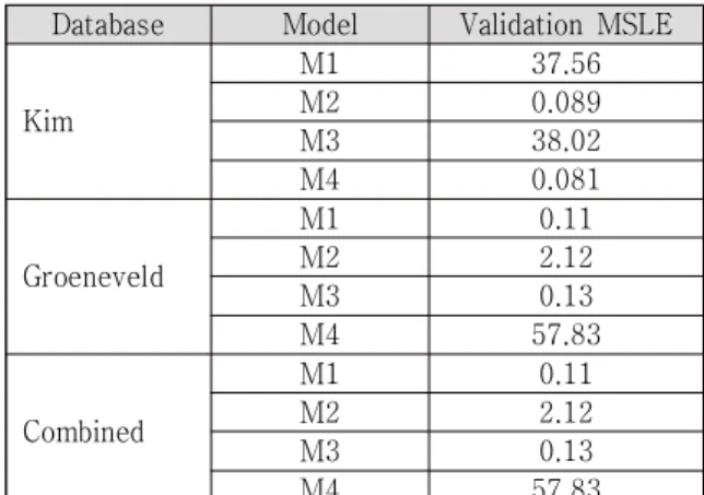
The developed model will be evaluated further by the built in evaluation function from the Scikit learn library to test the ANN performance. The evaluation function uses the MSLE metric to evaluate the model performance. Table 4 compares the overall performance of the developed ANN models. M1 performed well with an MSLE of 0.11 for both the Groneveld’s and combined databases.
<Table 4> ANN model validation metrics
To assess the performance of the ANN approach, the predictions are compared to those obtained using the support vector machine (SVM) technique. Model M1 is selected as the basis of comparison given its good performance.
The SVM is optimized to predict the CHF using the grid search method based on genetic algorithm initializations. The SVM model details are omitted for brevity since the focus of this work is on the ANN model development.
Table 5 contrasts the MSLE metric for the ANN M1 and the SVM models. Clearly, the
Database Model Validation MSLE
Kim M1 37.56 M2 0.089 M3 38.02 M4 0.081 Groeneveld M1 0.11 M2 2.12 M3 0.13 M4 57.83 Combined M1 0.11 M2 2.12 M3 0.13 M4 57.83
ANN model outperforms the SVM model.
<Table 5> Performance validation metric
AI Method MSLE
ANN (Model M1) 0.10
Support Vector Machine (SVM) 3.43
Despite the fact that the SVM model is much faster compared to the ANN model since it is based on the classification of the data rather than learning it. The ANN model performs much better. This is because, ANN consists of interconnected layers of neurons which makes it better at predicting the non-linear correlations between the input and output data. On the other hand, the SVM performance is limited since it relies on a kernel with a number of samples equal to the support vectors size. Additionally, the accuracy of the ANN increases as the number of hidden layers increases. Hence, the ANN is much more suited to the problem at hand.
7.1.6 Model Predictions
Figure 10 shows the lower range of prediction for Kim’s dataset that covers only the low flow and low pressure conditions while Groeneveld’s and the combined dataset cover a wider range of flow conditions as shown in Figures 11 and 12. The scatter plots illustrate the accuracy of model predictions, particulalry for Groeveld’s and combined databases since almost all the predictions lie on the 45 degree line that represents the equality between the predicted value and the known value of the CHF. Based on the results, we conclude that the CHF can be predicted with reasonable accuracy using ANN.
[Figure 10] Kim’s database prediction
[Figure 11] Groeneveld’s database prediction
[Figure 12] Combined database prediction
8. Conclusion
A System Engineering approach is successfully applied in this study to develop an ANN model capable of predicting the CHF for a set of flow conditions. The ANN model is
developed using Kossiakoff’s approach by breaking down the complex work structure to basic workable units. The developed model accurately predicted the CHF for different flow conditions using the pre-existing databases. This is the first step of an ongoing research effort to use the ANN model to predict the DNBR under design basis accident condition, for example large break LOCA.
Acknowledgement
This research was supported by the 2020 Research Fund of the KEPCO International Nuclear Graduate School (KINGS), Republic of Korea.
References
1. D. Groeneveld, "Critical Heat Flux Data Used," Office of Nuclear Regulatory Research, Ontario, 2019.
2. C. E. Nwankpa, "Activation Functions: Comparison of Trends in Practice and Research for Deep Learning," arXiv, 2018.
3. L. N. B, "Towards a Nuclear Industry Boosted by Artificial Intelligence," INIS International Nuclear Information System, pp.24-26,2017. 4. H. C. Kim, "Critical Heat Flux of Water in
Vertical Round Tubes at Low Pressure and Low Flow Conditions," Nuclear Engineering and Design, pp. 49-73,2000.
5. S. H. Chang, "Evaluation of Very High CHF for Subcooled Flow Boiling Using an Artificial Neural Network and Mechanistic Models," Proceedings of the Korean Nuclear Society Autumn Meeting, pp. 1-13, 2000.
6. G. Su, "Application of an Artificial Neural
Network in Reactor Thermohydraulics," Journal of Nuclear Science and Technology, pp. 564-571, 2002.
7. A. Kossiakoff, "Systems Engineering Principles and Practice," in Systems Engineering Principles and Practice Second Edition, New Jersey, A John Wiley & Sons Publication, 2011. 8. "What is a Stakeholder?," Corporate Finance Society, 2015. [Online]. Available at: https://corporatefinanceinstitute.com/resources/ knowledge/finance/stakeholder/.
9. A. Talos, "Autonomio/talos," Talos autonomy,
2019. [Online]. Available at:
https://github.com/autonomio/talos.
10. W. Wu, "Protocol for Developing ANN Models and its Application to the Assesment of the Quality of the ANN Model Development Process in Drinking Water Quality Modelling," Environmental Modelling & Software, pp. 108-127, 2014.
11. S. Kumar, "Data Splitting Technique to Fit any Machine Learning Model," 2019. [Online]. Available at:
https://towardsdatascience.com/data-splitting -technique-to-fit-any-machine-learning-model-c0d7f3f1c790.
12. H. M. Park, "Wall Temperature Prediction at Critical Heat Flux using a Machine," Annals of Nuclear Energy, pp. 1-9, 2020.
13. USNRC, "United States Nuclear Regulatory Commission," 26 June 2020. [Online]. Available:
https://www.nrc.gov/reading-rm/basic-ref/glo ssary/departure-from-nuclear-boiling-ratio -dnbr.html.