Model Predictive Control of Traffic Flow Based on Hybrid System Modeling

(1)

ICCAS2005 June 2-5, KINTEX, Gyeonggi-Do, Korea

Model Predictive Control of Traffic Flow Based on Hybrid System Modeling

Tatsuya Kato∗_{,YoungWoo Kim}∗∗_{and Shigeru Okuma}∗

∗_{Dept. of Information Electronics, Nagoya University, Nagoya, Aichi, Japan}

(Tel: +81-52-789-2777; e-mail: [email protected] Tel: +81-52-789-2775; e-mail: [email protected])

∗∗_{, Space Robotics Research Center, Toyota Technological Institute , Nagoya, Aichi, Japan}

(Tel: +81-52-809-1818; e-mail: [email protected])

Abstract: This paper presents a new framework for the traffic flow control based on integrated model descriptions as the Hybrid Dynamical System (HDS).

Keywords: Traffic Control,Mixed Logical Dynamical Systems ,Hybrid Petri Net

1. Introduction

With the increasing number of automobile and complication of traffic network, the traffic flow control becomes one of the significant economic and social issues in urban life. Many researchers have been involved in related researches in order to alleviate the traffic congestion.

Although this model expresses well the behavior of the flow on the freeway, it is unlikely that this model is also appli-cable to the urban traffic network which involves many dis-continuities of the density coming from the existence of the intersection controlled by the traffic signals.

This paper presents a new method for the real-time traffic signal control based on integrated model descriptions as the Hybrid Dynamical System (HDS). The geometrical informa-tion on the traffic network is characterized by using Hybrid Petri Net (HPN) by both graphical and algebraic descrip-tions. Then, the algebraic behavior of traffic flow is trans-formed into the Mixed Logical Dynamical Systems (MLDS) form in order to introduce the optimization technique.

2. Modeling of Traffic Flow Control System (TFCS) based on HPN

The Traffic Flow Control System (TFCS) is the collective entity of the traffic network, traffic flow and traffic signals. Although some of them have been fully considered by the previous studies, most of the previous studies did not simul-taneously consider all of them. In this section, the HPN model is developed, which provides both graphical and alge-braic descriptions for the TFCS.

2.1. Representation of TFCS as HPN

Sensor

Sensor SensorSensor SensorSensor SensorSensor SensorSensor SensorSensor Section 1 Section 2 Section 3 Section 4 Section 5

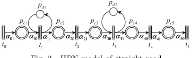
Fig. 1. Straight road

HPN is one of the useful tools to model and visualize the sys-tem behavior with both continuous and discrete variables. Figure 1 shows the HPN model for the road of Fig.2. In Fig.1, each section i of li-meter long constitutes the straight

1 c p pc2 pc3 pc4 pc5 1 d p pd2 0 t t₁ t2 t3 t4 t5 01 α01 α10 α11 α20 α21 α30 α31 α40 α41 α50 α α10 α11 α20 α21 α30 α31 α40 α41 α50 Fig. 2. HPN model of straight road

road, and two traffic lights are installed at the point of cross-walk. HPN has a structure of N = (P, T, q, I+, I−, M0). The

set of places P is partitioned into a subset of discrete places Pdand a subset of continuous places Pc. pc∈ Pcrepresents

each section of the road, and has maximum capacity (maxi-mum number of cars). Also, Pd represents the traffic signal

where green signal is indicated by a token in the correspond-ing discrete place pd∈ Pd. The marking M = [mC|mD] has both continuous (m dimension) and discrete (n dimension) parts where mC represents the number of vehicles in the correponding continuous places, and mD denotes the state of the corresponding traffic signal (i.e. takes binary value). Note that each signal is supposed to have only two states ‘go (green)’ or ‘stop (red)’ for the simplicity. T is the set of continuous transitions which represent the boundary of two successive sections. The function qj(τ ) specifies the firing

speeds assigned to transition tj ∈ T at time τ . qj(τ )

rep-resents the number of cars passing through the boundary of two successive sections (measuring position) at time τ . The functions I±(p, t) are forward and backward incidence

relationships between transition t and place p which con-nects the transition. The element of I(p, t) is always 0 or 1. Finally, M0 _{is specified as the initial marking of the place}

p ∈ P .

The net dynamics of HPN is represented by a simple first order differential equation for each continuous place pc_i∈ Pc

as follows : dmC,i(τ ) dt = X tj∈pci•∪•_p ci I(pci, tj) · qj(τ ) · mD,j(τ ) (1)

where mC,i(τ ) is the marking for the place pci(∈ Pc) at

time τ , mD,j(τ ) is the marking for the place pdj(∈ Pd), and

I(p, t) = I+(p, t) − I−(p, t). The equation (1) is transformed

(2)

during two successive sampling instants as follows : mC,i((κ + 1)Ts) = mC,i(κTs) + X tj∈pci•∪•_p ci I(pc_i, tj) · qj(κTs) · mD,j(κTs) · Ts (2)

where κ and Ts are sampling index and period.

Note that the transition t is enabled at the sampling instant κTs if the marking of its preceding discrete place pdj ∈ Pd

satisfies mD,j(κ) ≥ I+(pdj, t). Also if t does not have any

input (discrete) place, t is always enabled. 2.2. Definition of flow qi

In order to derive the flow behavior, the relationship among qi, kiand vimust be specified. One of the simple ideas is to

use the well-known model qi(τ ) = (ki(τ ) + ki+1(τ ))

2

vi(ki(τ )) + vi+1(ki+1(τ ))

2 (3)

supposing that the density k∗and average velocity v∗of the

flow in i and (i + 1)th sections are almost identical. Then, by incorporating the velocity model

vi(τ ) = vfi· µ 1 −ki(τ ) kjam ¶ (4) with (3), the flow dynamics can be uniquely defined. Here, kjamis the density in which the vehicles on the roadway are

spaced at minimum intervals (traffic-jammed), and vfi is the

free velocity, that is, the velocity of the vehicle when no other car exists in the same section.

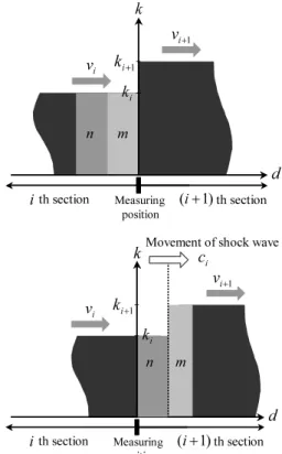
If there exist no abrupt change in the density on the road, this model is expected to work well. However, in the urban traffic network, this is not the case due to the existence of the intersections controlled by the traffic signals. In order to treat the discontinuities of the density among neighbor-ing sections (i.e. neighborneighbor-ing continuous places), the idea of ‘shock wave’[4] is introduced as follows. We consider the case as shown in Fig.3 where the traffic density of ith sec-tion is higher than that of (i + 1)th secsec-tion in which the boundary of density difference designated by the dotted line is moving forward. Here, the movement of this boundary is called shock wave and the moving velocity of the shock wave ci depends on the densities and average velocities of ith and

(i + 1)th sections as follows [4]:

ci(τ ) = vi(τ )ki(τ ) − vi+1(τ )ki+1(τ )

ki(τ ) − ki+1(τ ) (5)

The traffic situation can be categorized into the following four types taking into account the density and shock wave.

(C1) ki(τ ) < ki+1(τ ), and ci(τ ) > 0,

(C2) ki(τ ) < ki+1(τ ), and ci(τ ) ≤ 0,

(C3) ki(τ ) > ki+1(τ ),

(C4) ki(τ ) = ki+1(τ ) (no shock wave).

Firstly, in both cases of (C1) and (C2) where ki(τ ) is

smaller than ki+1(τ ), the vehicles passing through the

den-sity boundary (dotted line) reduce their speeds. The move-ment of the shock wave is illustrated in Fig.3 (ci(τ ) > 0) and

Fig.4 (ci(τ ) ≤ 0).

In Figs.3 and 4 , the ‘measuring position’ implies the po-sition where tranpo-sition ti is assigned. Since the traffic flow

) 1 ( +i i v 1 + i

v

Measuring position th section th section i k 1 + i

k

m

n i k

d

) 1 ( +i i v 1 + i v

d

Measuring position

th section

i

k

1 + i k i k

Movement of shock wave

i

c

m

n

Fig. 3. Movement of shock wave in the case of ki(τ ) <

ki+1(τ ) and ci(τ ) > 0

qi(τ ) represents the number of vehicle passing through the

measuring position per unit time, in the case of (C1), it can be represented by n + m in Fig.3, where n and m represent the area of the corresponding rectangular, i.e. the product of the viand ki. Similarly, in the case of (C2), qi(τ ) can be

represented by m in Fig.4. These considerations lead to the following models: in the case of (C1) qi(τ ) = vi(τ )ki(τ ) (6) = vfi µ 1 −ki(τ ) kjam ¶ ki(τ ) (7) in the case of (C2) qi(τ ) = vi+1(τ )ki+1(τ ) (8) = vfi+1 µ 1 −ki+1(τ ) kjam ¶ ki+1(τ ) (9)

In the cases of (C3) and (C4) where ki(τ ) is greater than

ki+1(τ ), the vehicles passing through the density boundary

come to accelerate. In this case, the flow can be well ap-proximated by taking into account the average density of neighboring two sections. This is intuitively because the dif-ference of the traffic density is going down. Then in the cases of (C3) and (C4), the traffic flow can be formulated as follows:

in the cases of (C3) and (C4), qi(τ ) = ³ ki(τ )+ki+1(τ ) 2 ´ vf(τ ) ³ 1 −ki(τ )+ki+1(τ ) 2kjam ´ (10)

(3)

) 1 ( +i i v 1 + i

v

Measuring position th section th section i k 1 + i

k

d

i k

m

n ) 1 ( +i i v 1 + i v Measuring position th section th section i k d i k 1 + i k Movement of shock wave

i c

m n

Fig. 4. Movement of shock wave in the case of ki(τ ) <

ki+1(τ ) and ci(τ ) ≤ 0 0 0.2 0.4 0.6 0.8 1 0 0.2 0.4 0.6 0.8 1 0 0.2 0.4 0.6 0.8 1

Traffic density of(

i )th section( ki ) Traffic density of ( i +1)th section( k i₊₁ ) Traffi flow( q i₎ B A C a b

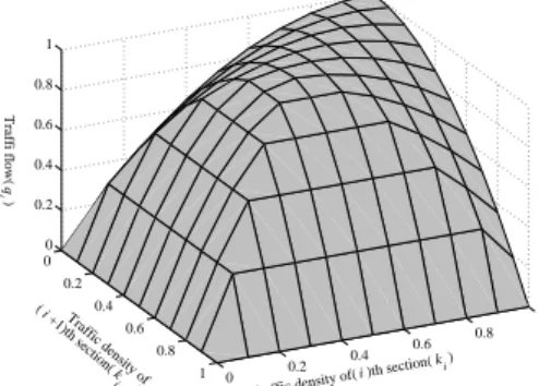
Fig. 5. Traffic flow behavior obtained from CA model

As the results, the flow model (6) ∼ (10) taking into ac-count the discontinuity of the density can be summarized as follows: qi(τ ) =                            ³ ki(τ )+ki+1(τ ) 2 ´ vf ³ 1 −ki(τ )+ki+1(τ ) 2kjam ´ if ki(τ ) ≥ ki+1(τ ) vfi ³ 1 −ki(τ ) kjam ´ ki(τ ) if ki(τ ) < ki+1(τ ) and c(τ ) > 0 vfi+1 ³ 1 −ki+1(τ ) kjam ´ ki+1(τ ) if ki(τ ) < ki+1(τ ) and c(τ ) ≤ 0 (11)

Figure 6 shows the traffic volume by proposed traffic flow model. We can see that the Fig.6 shows the similar charac-teristics to in Fig.5 that computed by Cellular Automaton (CA) model. 0 0.2 0.4 0.6 0.8 1 0 0.2 0.4 0.6 0.8 1 0 0.2 0.4 0.6 0.8 1

Traffic density of( i )th section( ki ) Traffic density of ( i +1)th section( k i+1) Traffi flow( q i₎

Fig. 6. Traffic flow behavior obtained from the proposed traffic flow model

3. Transformation to MLDS form

Although the HPN can represent the hybrid dynamical be-havior of the TFCS including both continuous traffic flow and discrete traffic signal control, it is still not well formu-lated when some optimization problem is addressed. In this section, the MLDS form is introduced to formulate the Model Predictive Control (MPC) stated in the next section. The MLDS form can generally be formalized as follows [6]:

x(κ + 1) = A»x(κ) + B1»u(κ) +B2»‹(κ) + B3»z(κ) (12) y(κ) = C»x(κ) + D1»u(κ) +D2»‹(t) + D3»(κ) (13) E2»‹(κ) + E3»z(κ) ≤ E1»u(κ) + E4»x(κ) + E5» (14) In the MLDS form,κ represents the sampling index. Note that sampling period Ts is eliminated the following.

Equa-tions (12), (13) and (14) are state equation, output equa-tion and constraint inequality, respectively, where x, y and u are the state, output and input variable, whose compo-nents are constituted by continuous and/or 0-1 binary vari-ables, δ(κ) ∈ {0, 1} and z(κ) ∈ < represent auxiliary logical (binary) and continuous variables. The MLDS is known to be able to represent other forms of HDS such as Piece-Wise Affine (PWA), Hybrid Automaton (HA) and so on.

In the TFCS represented by HPN, equation (2) is directly transformed to the state equation in MLDS form by regard-ing the continuous markregard-ing as the state. Also, the TFSC only has binary input variable which denotes the state of the traffic signal (i.e. green or red). The output variable is not specified in our problem setting since all states are supposed to be measurable in this work.

The constraint inequality of (14) often plays an essential role to represent some nonlinearity which exists in the original system. In the TFCS, the nonlinearity appears in (11). In the following, this nonlinear constraint is transformed to the set of linear inequality constraints. The flow model devel-oped in the previous section (shown in Fig.5) can be approx-imated by the Piece-Wise Affine (PWA) model shown in the right figure of Fig.5, which consists of three planes as follows: Plane A: The traffic flow qi is saturated (ki(κ) ≥ a and

(4)

1 + i

k

1 1 , ,i = P δ 1 2 , ,i = P δ a

k

i a kjam− 0 Traffic density of th section( ) i ki Traffic density of th section( ) i ki Tra ffic de ns ity o f th sec tio n ( ) 1+i 1+ ik Tra ffic de ns ity o f th sec tio n ( ) 1+i 1+ ik jam

k

1 3 , ,i = P δ jam

k

Fig. 7. Division of flow model by introducing auxiliary vari-ables

Plane B: The traffic flow qi is mainly affected by the

quantity of traffic density ki(κ) (ki(κ) < a and ki(κ) +

ki+1≤ kjam)

Plane C: The traffic flow qi is mainly affected by the

quantity of traffic density ki+1(κ) (ki+1(κ) > kjam− a

and ki(κ) + ki+1> kjam)

Here, a is the threshold value to specify the region of satu-ration characteristic of the traffic flow, that is, if ki(κ) ≥ a

and ki+1(κ) < kjam− a, the qi(κ) takes almost its maximum

value qmax.

Figure 7 shows this partitions on ki+1− ki plane. In order

to derive the linear inequalities expression of the flow model, three auxiliary variables δP,i,1(κ), δP,i,2(κ) and δP,i,3(κ) are

introduced, and are defined as follows: [δP,i,1(κ) = 1] ↔ ½ ki(κ) ≥ a ki+1(κ) ≤ kjam− a (15) [δP,i,2(κ) = 1] ↔ ½ ki(κ) ≤ a − ε ki(κ) + ki+1(κ) ≤ kjam (16) [δP,i,3(κ) = 1] ↔ ½ ki+1(κ) ≥ kjam− a + ε ki(κ) + ki+1(κ) ≥ kjam+ ε (17) δP,i,1(κ) + δP,i,2(κ) + δP,i,3(κ) = 1 (18)

where ε is a small tolerance.

By using these binary variables, the flow model qi(κ) given

by (11) can be rewritten in a compact linear form as follows: qi(κ) = qmaxδP,i,1(κ) +qmaxki(κ)

a δP,i,2(κ) +qmax(1 − ki+1(κ)) a δP,i,3(κ) (19) 3 X i=1 δP,i,j(κ) = 1

where 0 ≤ ki(κ) ≤ kjam, 0 ≤ ki+1≤ kjam(= 1), and qmax

is the maximum value of the traffic flow.

The equations (15) to (17) can be generalized as follows: [δP,i,j(κ) = 1] ↔ ·· ki ki+1 ¸ ∈ <j ¸ (20) <j = ½· ki ki+1 ¸ : Sjki(κ) ≤ Tj ¾ (21) where ki(κ) = [ki(κ) ki+1(κ)]T and Sj and Tj are the ma-trices with suitable dimensions. Also, this logical conditions can be transformed to inequalities

Sjki(κ) − Tj≤ Mj∗[1 − δP,i,j(κ)], (22) M˜ j 4 = max ki∈<j Sjki(») − Tj. (23) The flow qi(κ) of (19) can be represented by the vector form

by using

‹P;i(κ) = [δP,i,1(κ) δP,i,2(κ) δP,i,3(κ)] as follows:

qi(κ) = f (‹P;i(κ), ki+1(κ)) (24) = 3 X j=1 (f_ij(κ)ki(κ) + hj_i)δP,i,j(κ) (25) where fij and h j

i are given as follows (see Fig. 7):

f1 i = [ 0 0 ] , h1i = qmax (26) f2 i = [ qmaxa 0 ] , h 2 i = 0 (27) f3 i = [ 0 −qmaxa ] , h 3 i = qmax a (28)

Next, we introduce an auxiliary bariable ‘controlled traffic flow’ zi(κ) = [zi,1(κ) zi,2(κ) zi,3(κ)] which implies the flow

under the traffic signal control. zi,j(κ) is defined by

zi,j= (fij(κ)ki(κ) + hji)ui(κ)δP,i,j(κ). (29)

That is,

qiui= zi,1+ zi,2+ zi,3 (30)

where ui(κ) ∈ {0, 1} denotes the binary control input which

represents the state of the traffic signal. Then the equivalent inequalities to (29) is given as follows:

zi,j(κ) ≤ Miui(κ)δP,i,j(κ) (31) zi,j(κ) ≥ miui(κ)δP,i,j(κ) (32) zi,j(κ) ≤ fijki(κ) + hji −mi(1 − ui(κ)δP,i,j(κ)) (33) zi,j(κ) ≥ f_ijki(κ) + hj_i −Mi(1 − ui(κ)δP,i,j(κ)) (34)

where Miand miare

Mi = max ki(κ)∈<j © fijki(κ) + hji ª (35) mi = min ki(κ)∈<j © f_ijki(κ) + hji ª (36) The product term ui(κ) δP,i,j(κ) can also be replaced by

(5)

As the results, the MLDS form for the TFCS can be formal-ized as follows: x(κ + 1) = Ax(κ) + Bz(κ) (37) z(κ) = diag(Cu(κ))‹(κ) (38) E2‹(κ) + E3z(κ) ≤ E1u(κ) + E4x(κ) + E5 (39) where the element xi(κ) of x(κ) ∈ <|P |, is marking of the

place pciat the sampling index κ, the element ui(κ)(∈ {0, 1})

of u(κ) ∈ Z|T |_{, is the state of the traffic signal installed at}

ith section and ‹(κ)=[‹P(κ), ‹M(κ)]

0

. Note that if there is no traffic signal installed at ith section, ui(κ) is always set

to be one. E1, E2, E3, E4 and E5 of Fig.2 are described in the appendix.

4. Model Predictive Control for TFCS

The Model Predictive Control (MPC) [7]is one of the well-known paradigms for optimizing the systems with con-straints and uncertainties. The Receding Horizon Control (RHC) policy is the key idea to realize the MPC. In the RHC, finite-horizon optimization is carried out based on the measured state at each sampling instant, and only the first control input is applied to the controlled plant. In this sec-tion, firstly, the RHC policy is briefly reviewed, then the op-timization problem for the TFCS is formulated as the Mixed Integer Linear Programming (MILP). Finally, some idea to reduce the computational amount is described.

4.1. RHC for TFCS

In RHC policy, the control input at each sampling instant is decided based on the prediction of the behavior for next several sampling periods called the prediction horizon. In order to formulate the optimization procedure, firstly, equation (37) is modified to evaluate the state and input variables in the prediction horizon as follows:

x(κ + λ|κ) = A»_x(κ) + λ−1 X η=0 {A”_{(B(diag(Cu(κ + λ − 1 − η|κ)))} ·‹(κ + λ − 1 − η|κ))} (40) where x(κ + λ|κ) denotes the predicted state vector at sam-pling index κ + λ, which is obtained by applying the input sequence, u(κ), · · · , u(κ + λ) to (37) starting from the state x(κ|κ) = x(κ).

Now we consider the following control requirements that usu-ally appear in the TFCS.

(R1) Maximize the traffic flow over entire traffic network (R2) Avoid the frequent change of traffic signal

(R3) Avoid the concentration of traffic mass in a certain section

These requirements can be realized by minimizing the fol-lowing objective function.

N denotes the prediction horizon. Also, w1,i, w2,i and w3,i are positive weighting parameters for ith section which sat-isfy w1,i+ w2,i+ w3,i= 1, and 0 ≤ w1,i≤ 1, 0 ≤ w2,i≤ 1 and 0 ≤ w3,i ≤ 1. The three terms in the left side of (41) correspond to the requirement (R1), (R2) and (R3), respec-tively.

As the results, the optimization problem can be formulated as follows: f ind ‹(» + –j») = [ ‹P(» + –j»), ‹M(» + –j») ] 0 (λ = 1, · · · N ) which minimizes (41) subject to (22), (23),(26) ∼ (28),and (30) ∼ (39)

The MLDS formulation coupled with RHC scheme can be transformed to the canonical form of 0-1 Mixed Integer Lin-ear Programming (MILP) problem with the objective func-tion of (41). As the solver for the MILP, we have adopted the Branch-and-Bound (B&B) algorithm.

5. Numerical experiments

5.1. Signal control in intersections

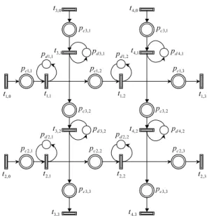
In this section, we consider the signal control for the traffic network as shown in Fig. 8. This traffic network consists of four intersections, however, only the single-way of the traf-fic flow is allowed on each road. We assume that each car comes in from left side of this network every 30 seconds, and comes in from top side every 100 seconds. This implies that the horizontal traffic flow has higher amount than the ver-tical traffic flow. We have examined following four control conditions.

1. change the signal every 30 seconds (no control) 2. MPC with Prediction Horizon N = 1

3. MPC with Prediction Horizon N = 4 without consid-eration of uniformity of traffic density (w3was set to be zero)

4. MPC with Prediction Horizon N = 4 with considera-tion of uniformity of traffic density

CA was used to simulate the movement of each car. Table 1 shows the total number of cars which pass through this traffic network in both horizontal and vertical directions.

(6)

3 , 1 t 0 , 1 t t1,1 t1,2 3 , 2 t 0 , 2 t t2,1 t2,2 0 , 3 t 1 , 3 t 2 , 3 t 3 , 3 t 0 , 4 t 1 , 4 t 2 , 4 t 3 , 4 t 1 , 1 c p pc1,2 pc1,3 1 , 2 c p pc2,2 pc2,3 1 , 3 c p 2 , 3 c p 3 , 3 c p 1 , 3 c p 2 , 3 c p 3 , 3 c p 1 , 1 d p pd1,2 1 , 2 d p pd2,2 1 , 3 d p 2 , 3 d p 1 , 4 d p 2 , 4 d p

Fig. 8. HPN of traffic network with four single-way inter-sections

Table 1. Results of the intersection control

Control Conditions 1 2 3 4

Number of passing cars 18 41 56 58

Rate of Green signal

in left to right road(%) 50 65.2 88.5 87.5

From these results, we can see that the MPC with longer pre-diction horizon enables more cars to get through this traffic network. Also, evaluations of the computational efforts are shown in Fig. 9.

1. Branch-and-Bound method 2. full search method

Here, ”full search method” implies the algorithm where 0-1 combinations are directly allocated to the binary variables, and quadratic programming is applied in order to optimize the continuous variables. The optimal solution is found based on the performance criterion. From Fig.9, we can see that the difference of the computational efforts between two schemes becomes larger as the increase of the horizon.

0 2 4 6 8 10-2 100 102 104 106 108

Size of Problem (Horizen)

Computational Time (Sec)

branch and bound full search

Fig. 9. Computational efforts

6. Conclusions

In this paper, we have proposed a new method for traffic sig-nal control based on hybrid dynamical system theory. First of all, the synthetic modeling method for the Traffic Flow Control System (TCCS) has been proposed where the infor-mation on geometrical traffic network was modeled by us-ing Hybrid Petri Net (HPN), whereas the information on the behavior of traffic flow was modeled by means of Mixed Logical Dynamical Systems (MLDS) form. The former al-lows us to easily apply our method to complicated and wide range of traffic network due to its graphical understanding. The latter enables us to optimize the control policy for the traffic signal by means of its algebraic manipulability and use of model predictive control framework. Secondly, the shock wave model has been introduced in order to treat the discontinuity of the traffic flow. By approximating the de-rived flow model with piece-wise linear function, the flow model has been naturally coupled with the MLDS form. Fi-nally, the model predictive control problem for the TFCS has been formulated. This formulation has been recasted to the 0-1 Mixed Integer Linear Programming (MILP) problem. Some numerical experiments have been carried out, and have shown the usefulness of the proposed design framework.

References

[1] S.Darabha and K.R.Rahagopal ”Intelligent cruise con-trol systems and traffic flow stabilityhTransportation Re-search Part C 7(1999) 329-352

[2] K. Nagel and M. Schreckenberg. A Cellular Automaton Model for Freeway Traffic. Journal de Physique I France, 2: 2221, 1992.

[3] First-order hybrid Petri nets: a model for optimization and control. , IEEE Trans. on Robotics and Automation, Vol. 16, No. 4, pages 382-399. 2000.

[4] Richard Haberman Mathematical Models

[5] Chaudahuri, P.P, et al. : Additive Cellular Automata - Theory and Applications, IEEE Computer Society Press(1997)

[6] A. Bemporad, M. Morari, ” Control of systems integrat-ing logic, dynamics, and constraints”, Automatica, Vol. 35, n. 3, p. 407-427, 1999.

[7] M. Morari ; E. Zafirou. Robust Process Control. Prentice Hall, 1989.