Article
Structural Changes in the Korean Housing Market
before and after Macroeconomic Fluctuations
Sanghyun Kim, Juhyung Kim and Jaejun Kim *
Department of Architectural Engineering, Hanynag University, 222,Wangsipri-ro, Sungdong-gu, Seoul 133-791, Korea; [email protected] (S.K.); [email protected] (J.K.)
* Correspondence: [email protected]; Tel.: +82-2-2220-0307; Fax: +82-2-2296-1583 Academic Editor: Vincenzo Torretta
Received: 8 March 2016; Accepted: 19 April 2016; Published: 27 April 2016
Abstract:The purpose of this paper is to identify structural changes in the Korean housing market for evaluating the sustainability of the Korean housing market and to derive important implications to seek housing business strategies and public policies. Two time periods were analyzed: April 2001–December 2007 and January 2008–December 2014 to identify the impact after the global financial crisis of 2008. The market was divided into transaction, chonsei, and monthly rent. The correlations were analyzed using a vector error correction model (VECM). A key result was that during the economic depression, demand for chonsei did not flow to the transaction market; this phenomenon affected the overall recovery of the housing market. The supply of chonsei today is rapidly decreasing with the depression in the transaction. Increases in chonsei prices are expected to continue along with the possibility that demand for chonsei will flow into the transaction or monthly rent market. Based on recent trends, the chonsei market, once main stream, will gradually weaken, and the Korean housing market will reorganize into transactions and monthly rent. This structural change may turn the Korean housing market into a target for long-term investments.
Keywords: Korean housing market; macroeconomics fluctuation; Fisher–Dipasquale–Wheaton model; vector error correction model
1. Introduction
As the subprime mortgage crisis spread globally, it depressed not only the financial market but also the construction business in Korea. In fact, according to an announcement from the Construction & Economy Research Institute of Korea (CERIK), the Business Survey Index (BSI) of construction businesses plunged from 80points in December 2006 to 14.6points in November 2008, and the extent of the depression in the housing sector was particularly serious. Before the financial crisis, house owners bought houses using loans under the expectation that housing prices would rise, and, as prices dropped and the housing transaction market shrank, household debts rapidly increased. In addition, as the housing market entered a decline after the financial crisis with the selling prices falling, the burden on rental tenants increased as monthly rental fees increased. Due to such macroeconomic fluctuations, the housing market system in Korea has also changed.
In Korea, there is a unique way of renting a house, called chonsei. The tenant pays an upfront lump-sum deposit, which is typically from 40% to 70% of the property value, to the landlord for the use of the property. The landlord repays the nominal value of the deposit to the tenant upon contract termination. There is no additional requirement for the tenant such as periodic rental payments. Thus, the chonsei deposit, which is held during the contract period and repaid by the landlord, is the substitute for such payments [1].
The Korean housing market has a different structure than other overseas housing markets generally comprised of a transaction market and a monthly rent market. This is precisely because the
market share of the chonsei market in Korea is very high. The main feature of the chonsei market is that landlords can lower their capital investments considerably when buying houses. At the time, if a landlord buys a house borrowing money at market interest rates, which will be paid back using the chonsei deposit from the tenant, and then pursues a profit by selling the house at an increased price, the deposit functions as leverage for the landlord. In the meantime, for the tenant, the deposit functions as a reserve fund for buying a house in the future while also being used as a means to having a residence for two years [1,2].
As a result of macroeconomic fluctuations and this particular chonsei market aspect, the Korean housing market is presumed to have gone through unique structural changes compared to other overseas housing markets. Accordingly, analyzing the characteristics of the dynamic relationship between the transaction market, the chonsei market, and the monthly rent market before and after macroeconomic fluctuations could be very important in evaluating the sustainability of the Korean housing market and seeking housing business strategies and policies.
In this respect, this study intends to identify the structural changes in the Korean housing market for evaluating the sustainability of the Korean housing market and derive the implications to seek housing business strategies and public policies by dividing the Korean housing markets into transaction, chonsei, and monthly rent markets, and analyzing the dynamic relationships between these using a vector error correction model (VECM). In this study, data from the Seoul apartment market, which is a representative housing market in Korea, were utilized. The temporal range of the time series data was divided into two periods. The first period is from April 2001 to December 2007, the period prior to the financial crisis, set as Period A, and, the second period is from January 2008 to December 2014 and set as Period B. The time series data are from the Statistics Korea database. 2. Background
2.1. Changes in the Korean Housing Market
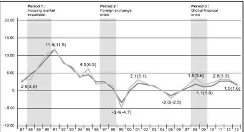
To identify the structural changes in the Korean housing market caused by recent macroeconomic fluctuations, aspects of overall change in the Korean housing market were first identified—that is, the changes in the housing market were identified by investigating three time periods: housing market expansion (1988 to 1990), foreign exchange crisis (1997 to 1999), and global financial crisis (2008 to 2009).
The first period represents housing market changes that started when the Korean housing market was expanding (1988 to 1990). During the first period investigated (1988–1990), by successfully achieving economic growth through industrialization, Korea recorded a rapid increase in income and a large-scale surplus balance in international trade. Urban concentration was accelerated by such industrialization, and the increase in the urban population eventually aggravated a shortage in housing. Accordingly, as shown in Figures1–3housing transaction prices, chonsei prices and monthly rental fees rapidly increased. As the housing market overheated, the government enforced powerful anti-speculation policies, such as supply expansion and tax reinforcement, in the real estate market. Subsequently, the whole housing market maintained a stable downward trend until 1996, before the outbreak of the foreign exchange crisis.
The second period represents the housing market changes during the time of the foreign exchange crisis (1997 to 1999). In this period, both the financial market and the real estate market stagnated due to the economic recession resulting from this unprecedented economic crisis, which began in 1997. Moreover, as shown in Figures1–3not only the housing transaction market but also the housing chonsei and the monthly rental market were depressed by the foreign exchange crisis. However, as the overall housing transaction market was invigorated from housing market policies of the government, the housing chonsei market also started to recover. In addition, from 2004 to 2005, while house prices increased, monthly rents fell significantly more than housing chonsei prices due to shrinking demand in the rent market.
The third period represents the housing market changes during the time of the global financial crisis (2008 to 2009). The global financial crisis, which began in 2008, acted as an important turning point in the housing market. As shown in Figure1, the housing transaction market was depressed by the global financial crisis. As the government had already witnessed an abnormal overheating phenomenon in the real estate market in the recent past, resulting from the economic invigoration policy enforced after the foreign exchange crisis, it did not pursue such a powerful real estate invigoration again. As a result, a differentiation in the housing market by district occurred. That is, although housing transaction prices in Seoul, which had previously foreshadowed the housing market trends in the whole country, continued to drop, housing transaction prices in provincial areas rose. However, the current Korean housing market is in a stagnant state due to the shrinking investment psychology. Though the housing transaction market was very seriously affected by the global financial crisis, as shown in Figures2and3the effects on the housing chonsei and monthly rental market were found to be relatively small. Moreover, housing chonsei prices and monthly rents maintained a continuous increasing trend after 2010.
Sustainability 2016, 8, 415 3 of 19 The third period represents the housing market changes during the time of the global financial crisis (2008 to 2009). The global financial crisis, which began in 2008, acted as an important turning point in the housing market. As shown in Figure 1, the housing transaction market was depressed by the global financial crisis. As the government had already witnessed an abnormal overheating phenomenon in the real estate market in the recent past, resulting from the economic invigoration policy enforced after the foreign exchange crisis, it did not pursue such a powerful real estate invigoration again. As a result, a differentiation in the housing market by district occurred. That is, although housing transaction prices in Seoul, which had previously foreshadowed the housing market trends in the whole country, continued to drop, housing transaction prices in provincial areas rose. However, the current Korean housing market is in a stagnant state due to the shrinking investment psychology. Though the housing transaction market was very seriously affected by the global financial crisis, as shown in Figures 2 and 3, the effects on the housing chonsei and monthly rental market were found to be relatively small. Moreover, housing chonsei prices and monthly rents maintained a continuous increasing trend after 2010.
Figure 1. Rates of changes in housing transaction prices for the country and Seoul.
Figure 2. Rates of the change in housing chonsei prices of the country and Seoul. Figure 1.Rates of changes in housing transaction prices for the country and Seoul.
Sustainability 2016, 8, 415 3 of 19 The third period represents the housing market changes during the time of the global financial crisis (2008 to 2009). The global financial crisis, which began in 2008, acted as an important turning point in the housing market. As shown in Figure 1, the housing transaction market was depressed by the global financial crisis. As the government had already witnessed an abnormal overheating phenomenon in the real estate market in the recent past, resulting from the economic invigoration policy enforced after the foreign exchange crisis, it did not pursue such a powerful real estate invigoration again. As a result, a differentiation in the housing market by district occurred. That is, although housing transaction prices in Seoul, which had previously foreshadowed the housing market trends in the whole country, continued to drop, housing transaction prices in provincial areas rose. However, the current Korean housing market is in a stagnant state due to the shrinking investment psychology. Though the housing transaction market was very seriously affected by the global financial crisis, as shown in Figures 2 and 3, the effects on the housing chonsei and monthly rental market were found to be relatively small. Moreover, housing chonsei prices and monthly rents maintained a continuous increasing trend after 2010.
Figure 1. Rates of changes in housing transaction prices for the country and Seoul.
Figure 2. Rates of the change in housing chonsei prices of the country and Seoul. Figure 2.Rates of the change in housing chonsei prices of the country and Seoul.
Figure 3. Rates of change in monthly rent of the country and Seoul.
2.2. Literature Review
Structural changes in the housing market are often generated by changes in the demand and supply of houses. There has been abundant literature that has analyzed the diverse factors that have an effect on the demand and supply sides of the housing market. The literature related to the housing demand mainly features studies on the motives behind house purchase, the financing ability, and analysis of housing price elasticity in view of housing demand. Green et al. measured the impact of age, education, and income on the willingness of households to pay for a consistent quality house [3]. Nordvik analyzed housing demand as a dynamic plan, which depended on the expected time‐path of moving costs and prices of housing consumption over the lifecycle [4]. Ahmad estimated demand for housing and its attributes in urban Bangladesh using a survey of 4400 owner, renter, and squatter households. This study showed that housing demand was elastic with respect to income and price; and price elasticity was less than income elasticity in absolute terms [5]. Goodman provided a discrete‐time consumer optimization model with transaction costs. This study indicated that income and value‐rent measures in different years had separable and significant impacts on housing demand [6]. Hansen et al. developed a new approach to the estimation of income elasticity and the demand for housing. This study provided evidence of substantial variation in elasticity across income classes [7].
The literature related to housing supply largely features studies on the relation between the housing supply and housing market, the issue of controlling the housing supply depending on changes in the housing market, and analysis of the housing price elasticity from the perspective of housing supply. Ooi et al. looked at Singapore between 1996 and 2009 and traced the price response of existing houses to the quantity of new units launched by home builders [8]. Malpezzi et al. estimated the price elasticity of the housing supply from new construction separately in the United States and in the United Kingdom [9]. Harter‐Dreiman also provided information about the price elasticity of the housing supply. The study suggested an elastic long‐run supply function but a relatively slow pace adjustment to the long‐run equilibrium [10]. Glaeser et al. presented a simple model of housing bubbles that predicted that places with more elastic housing supply had fewer and shorter bubbles, with smaller price increases. This study showed that the price run‐ups of the 1980s were almost exclusively experienced in cities where housing supply was more inelastic [11]. Paciorek examined the strong relationship between the volatility of house prices and the regulation of new housing supply. This study found that supply constraints increased volatility through two channels: first, regulation lowered the elasticity of new housing supply by increasing lags in the permit process and adding to the cost of supplying new houses on margin; second, geographic limitations in the area available for building houses, such as steep slopes and water bodies, led to
Figure 3.Rates of change in monthly rent of the country and Seoul.
2.2. Literature Review
Structural changes in the housing market are often generated by changes in the demand and supply of houses. There has been abundant literature that has analyzed the diverse factors that have an effect on the demand and supply sides of the housing market. The literature related to the housing demand mainly features studies on the motives behind house purchase, the financing ability, and analysis of housing price elasticity in view of housing demand. Green et al. measured the impact of age, education, and income on the willingness of households to pay for a consistent quality house [3]. Nordvik analyzed housing demand as a dynamic plan, which depended on the expected time-path of moving costs and prices of housing consumption over the lifecycle [4]. Ahmad estimated demand for housing and its attributes in urban Bangladesh using a survey of 4400 owner, renter, and squatter households. This study showed that housing demand was elastic with respect to income and price; and price elasticity was less than income elasticity in absolute terms [5]. Goodman provided a discrete-time consumer optimization model with transaction costs. This study indicated that income and value-rent measures in different years had separable and significant impacts on housing demand [6]. Hansen et al. developed a new approach to the estimation of income elasticity and the demand for housing. This study provided evidence of substantial variation in elasticity across income classes [7].
The literature related to housing supply largely features studies on the relation between the housing supply and housing market, the issue of controlling the housing supply depending on changes in the housing market, and analysis of the housing price elasticity from the perspective of housing supply. Ooi et al. looked at Singapore between 1996 and 2009 and traced the price response of existing houses to the quantity of new units launched by home builders [8]. Malpezzi et al. estimated the price elasticity of the housing supply from new construction separately in the United States and in the United Kingdom [9]. Harter-Dreiman also provided information about the price elasticity of the housing supply. The study suggested an elastic long-run supply function but a relatively slow pace adjustment to the long-run equilibrium [10]. Glaeser et al. presented a simple model of housing bubbles that predicted that places with more elastic housing supply had fewer and shorter bubbles, with smaller price increases. This study showed that the price run-ups of the 1980s were almost exclusively experienced in cities where housing supply was more inelastic [11]. Paciorek examined the strong relationship between the volatility of house prices and the regulation of new housing supply. This study found that supply constraints increased volatility through two channels: first, regulation lowered the elasticity of new housing supply by increasing lags in the permit process and adding to the cost of supplying new houses on margin; second, geographic limitations in the area available for building houses, such as steep slopes and water bodies, led to less investment, on average, relative
to the size of the existing housing supply, leaving less scope for the supply response to attenuate the effects of a demand shock [12].
The dynamics of the housing market that appear along with such demand/supply movements vary depending on the market characteristics of each region. Thus, researchers from diverse regions have studied the dynamics of their housing markets. In such cases, the focus was on grasping the long- and short-term movements of the housing market, taking into account various factors such as macroeconomic fluctuations, and population change. Englund et al. compared the dynamics of housing prices in 15 OECD countries [13]. Kenny attempted to model the demand and supply sides of the Irish housing market within an econometric framework, which clearly distinguished the long-from the short-run information among a relevant set of economic variables. This study suggested significant constraints on the supply side of the market and the potential for house prices to overshoot their long-run equilibrium following a sudden increase in housing demand [14]. Sing et al. empirically tested house price dynamics associated with the mobility of households in the public resale and private housing markets in Singapore. The results of this study supported the hypothesis that household mobility created co-movements of prices in public and private housing submarkets in the long run [15]. Jud et al. examined the dynamics of real housing price appreciation in 130 metropolitan areas across the United States. This study found that real housing price appreciation was strongly influenced by the growth of the population and real changes in income, construction costs, and interest rates [16].
Similarly, there have also been many studies on structural changes in the Korean housing market. In particular, as the Korean housing market expanded very quickly as a result of rapid economic growth and the unique housing chonsei market existed, there was some literature that derived significant implications. Cho et al. identified the long-term relationship between housing values and interest rates in the Korean housing market using a co-integration test and spectral analysis. This study showed a long-term negative equilibrium relationship between housing values and interest rates [17]. Kim showed why chonsei contracts exist and have been popular in Korea. This study showed that chonsei contract was an ingenious market response in an era of financial repression in Korea, allowing landlords to accumulate sufficient funds for housing investment without major reliance on mortgages [1]. Kim explored the nexus between housing and the Korean economy and arrived at a brief assessment of the government’s intervention to stabilize housing prices [18]. Hwang et al. presented very powerful panel tests of the dividend pricing relation using a unique data set in which dividends were set by market forces independent of managers’ preferences [19]. Ambrose et al. discussed the development and popularity of this contractual agreement in the context of public policy initiatives and historical and institutional settings surrounding the Korean housing and housing finance markets [2]. Park et al. utilized a qualitative system dynamics model to elucidate and investigate complex Korean housing mechanisms [20]. Holmes et al. examined long-run house price convergence across US states using a pair-wise approach. This study showed that long-run house price convergence was present across US states and Metropolitan [21]. Holmes et al. examined long-run house price convergence across the twenty Paris districts using a quarterly dataset that spans from 1991 to 2014. This study suggested that smaller distances between Parisian districts were associated with a faster speed of adjustment back towards long-run equilibrium [22].
However, though there was a structural change in the Korean housing market after the recent rapid macroeconomic fluctuations, there was a limit in empirically analyzing this. For this reason, in this paper, we intend to derive implications by analyzing the structural changes in the Korean housing market before and after the global financial crisis in 2008 using the vector error correction model (VECM).
2.3. Vector Auto Regression (VAR) Model
Each individual macroeconomic variable is not independent but has correlations with and an effect on other variables. The VAR model can practically use valuable information without losing any, as there is no restriction to a specific economic theory imposed on the structural relation between the
model’s variables. That is, the VAR model can be a dynamic model where variables influence each other in the analysis of several time series data.
The VAR model is comprised of n linear regression equations; each equation sets the current observations of each variable having a casual relation with it as dependent variables and the past observations of it and other variables as explanatory variables. In general, the VAR model, where the time difference is p for N ¨ 1 (vector) of the macroeconomic variables Yt, can be expressed in the following regression equation:
Y “ α0` n ÿ i“1
αtYt´1`et (1)
Here, Ytis N ¨ 1 (vector) of the macroeconomic variables, αtis the coefficient matrix, etis the random error, and L is the time difference operator and represents L1Yt= Yt´1, L2Yt= Yt´1, ¨¨¨, A(L) = A1L1+ A2L2+ A3L3. However, when the time series data of the VAR model are unstable, the level variables are differenced and utilized for the analysis, at which time the level variables’ unique information can be lost. In such a case, if a long-term linear relation, that is, co-integration, exists between the unstable level variables, the analysis can be conducted utilizing the vector error correction model (VECM). The VECM is a limited form of the VAR model used in the case when co-integration exists, and is a dynamic model in which the co-integration relation between the time series is taken into account along with other short-term dynamic relations, which can be written as follows:
∆Xt“ p´1
ÿ i“1
Γi∆Xt´i` αβ1Xt´p`ui (2)
B is a (n ˆ r) matrix that shows a co-integration relation. The term β’Xt´p, which is a linear combination of r items, represents the disequilibrium error at the point in time t´p and this disequilibrium error comes to have an effect on {Xt} at the next point in time t through the coefficient α. For this reason, the (n ˆ r) coefficient matrix α is called an error correction coefficient. In this paper, a co-integration test was actually conducted, and, as the result showed that co-integration existed, the empirical analysis was conducted using the VECM.
3. Theoretical Framework
The Fisher-Dipasquale-Wheaton (FDW) model is a quadrant model that defines demand-supply equilibrium in the real estate market and traces the relation between the space market and the asset market [23,24].
There are two types of links between the asset market and space market. First, the level of rent determined in the space market determines the demand for the real underlying asset. Investors purchase real estate considering its current income or predicting its future income in general. That is, the changes in the rent in the space market have an immediate effect on the demand for assets in the capital market. Second, the volume of construction plays a role as an important link between the two markets. If the volume of construction increases, not only do prices drop in the asset market but also the rent fees drop in the space market. Such correlations between the space market and the asset market are shown in the quadrant model in Figure4below.
As shown in Figure4, though the basic FDW model is comprised of the relation between the space market and the asset market, in the case of the Korean housing market, the space market, which is a rental market, is classified into the housing chonsei market and the monthly rental market. In particular, the housing chonsei market is the unique rental market to Korea where the residential right to rent a space is secured by making a security deposit.
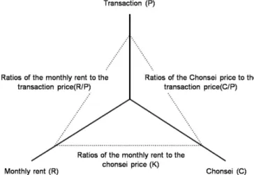
The structure of the Korean housing market comprised of the housing transaction market, the housing chonsei market, and monthly rental market can be expressed as shown in Figure5.
The three-dimensional model of the housing market is comprised of three axes’ transactions, chonsei, and monthly rent; the relation between the individual markets can be shown using the ratios
of the chonsei price to the transaction price, the monthly rent to the transaction price, and the ratios of the monthly rent to the chonsei price. Although moving independently, the individual markets are changed by factors in the housing market. These include: demand determinants such as the change in the number of households or income; supply determinants such as the increase in housing stock or decrease in construction volume; and, asset market factors such as the interest rate, the expectations of prospective buyers around rising prices, housing policy, and taxes.
Sustainability 2016, 8, 415 7 of 19 ratios of the monthly rent to the chonsei price. Although moving independently, the individual markets are changed by factors in the housing market. These include: demand determinants such as the change in the number of households or income; supply determinants such as the increase in housing stock or decrease in construction volume; and, asset market factors such as the interest rate, the expectations of prospective buyers around rising prices, housing policy, and taxes.
Figure 4. Fisher‐Dipasquale‐Wheaton (FDW) model.
Figure 5. Three‐dimensional structure of the Korean housing market. The market change caused by the fluctuation in the market interest rate is as shown in Figure 6 below. According to asset pricing theory, housing price can be defined as the asset value calculated by converting the monthly rent into the discounted rate of return on the capital investment. If it is assumed that the capitalization rate moves in the same direction as the market interest rate, the transaction price decreases and the monthly rent increases as the market interest rate increases. As shown in Figure 6, the transaction price moves from point p to p′ and monthly rent moves from r to r′ as the market interest rate increases from the initial state of equilibrium, and the ratio of monthly rent to the transaction price increases. At this time, though the chonsei price changes, as it is concurrently affected by the transaction price and the monthly rent, it is difficult to judge whether the direction of the change will be from c to c′ or from c to c″. This is because the chonsei price moves in the opposite direction to the market interest rate in relation to monthly rent and in the same direction as the market interest rate in relation to the transaction price.
Figure 4.Fisher-Dipasquale-Wheaton (FDW) model.
Sustainability 2016, 8, 415 7 of 19 ratios of the monthly rent to the chonsei price. Although moving independently, the individual markets are changed by factors in the housing market. These include: demand determinants such as the change in the number of households or income; supply determinants such as the increase in housing stock or decrease in construction volume; and, asset market factors such as the interest rate, the expectations of prospective buyers around rising prices, housing policy, and taxes.
Figure 4. Fisher‐Dipasquale‐Wheaton (FDW) model.
Figure 5. Three‐dimensional structure of the Korean housing market. The market change caused by the fluctuation in the market interest rate is as shown in Figure 6 below. According to asset pricing theory, housing price can be defined as the asset value calculated by converting the monthly rent into the discounted rate of return on the capital investment. If it is assumed that the capitalization rate moves in the same direction as the market interest rate, the transaction price decreases and the monthly rent increases as the market interest rate increases. As shown in Figure 6, the transaction price moves from point p to p′ and monthly rent moves from r to r′ as the market interest rate increases from the initial state of equilibrium, and the ratio of monthly rent to the transaction price increases. At this time, though the chonsei price changes, as it is concurrently affected by the transaction price and the monthly rent, it is difficult to judge whether the direction of the change will be from c to c′ or from c to c″. This is because the chonsei price moves in the opposite direction to the market interest rate in relation to monthly rent and in the same direction as the market interest rate in relation to the transaction price.
Figure 5.Three-dimensional structure of the Korean housing market.
The market change caused by the fluctuation in the market interest rate is as shown in Figure6 below. According to asset pricing theory, housing price can be defined as the asset value calculated by converting the monthly rent into the discounted rate of return on the capital investment. If it is assumed that the capitalization rate moves in the same direction as the market interest rate, the transaction price decreases and the monthly rent increases as the market interest rate increases. As shown in Figure6, the transaction price moves from point p to p1and monthly rent moves from r to r1 as the market interest rate increases from the initial state of equilibrium, and the ratio of monthly rent to the transaction price increases. At this time, though the chonsei price changes, as it is concurrently affected by the transaction price and the monthly rent, it is difficult to judge whether the direction of the change will be from c to c1or from c to c”. This is because the chonsei price moves in the opposite
direction to the market interest rate in relation to monthly rent and in the same direction as the market interest rate in relation to the transaction price.Sustainability 2016, 8, 415 8 of 19
Figure 6. Market change following the fluctuation in the interest rate.
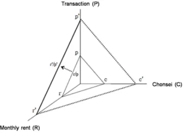
As the expected rate ofthe price increase relates to the expectations of investors that housing prices will rise or fall in the future, it is conceptually independent from monthly rent. In general, a rise in the expected rate of a price increase pushes up housing prices. However, the chonsei price moves in the opposite direction to the expected rate of the price increase in relation to the three markets. As the chonsei market is like the rent market and reflects the current flow of the housing supply, a rise in the expected rate of the price increase has the effect of decreasing the chonsei price.
Figure 7 shows the example where the transaction price increases from p to p′ and the chonsei price decreases from c to c′ as the expected rate of the price increase rises from its initial state of equilibrium.
Figure 7. Market change as a result of an increase in the expected rate of price increase.
At this time, if the monthly rent is fixed, as the ratio of the monthly rent to the chonsei price increases, this becomes a relatively bigger monthly rent when the chonsei deposit is converted into monthly rent in the rent market. The ratio of the chonsei price to the transaction price decreases from c/p to c′/p′. At the same time, the extent of change in c′/p′ varies depending on how sensitive the transaction price and the chonsei price are to the expected rate of the price increase. Accordingly, in the situation where price is expected to increase in the future, the chonsei price begins to drop in comparison to the transaction price.
The above discussion describes the theoretical view through an analysis of the relation of the individual markets. However, the movement of price in the actual market is affected by demand and supply determinants. If monthly rent increases due to a decrease in supply from a state of equilibrium, and other factors, such as the market interest rate, are unchangeable as in the FDW
Figure 6.Market change following the fluctuation in the interest rate.
As the expected rate ofthe price increase relates to the expectations of investors that housing prices will rise or fall in the future, it is conceptually independent from monthly rent. In general, a rise in the expected rate of a price increase pushes up housing prices. However, the chonsei price moves in the opposite direction to the expected rate of the price increase in relation to the three markets. As the chonsei market is like the rent market and reflects the current flow of the housing supply, a rise in the expected rate of the price increase has the effect of decreasing the chonsei price.
Figure7shows the example where the transaction price increases from p to p1and the chonsei price decreases from c to c1as the expected rate of the price increase rises from its initial state of equilibrium.
Sustainability 2016, 8, 415 8 of 19
Figure 6. Market change following the fluctuation in the interest rate.
As the expected rate ofthe price increase relates to the expectations of investors that housing prices will rise or fall in the future, it is conceptually independent from monthly rent. In general, a rise in the expected rate of a price increase pushes up housing prices. However, the chonsei price moves in the opposite direction to the expected rate of the price increase in relation to the three markets. As the chonsei market is like the rent market and reflects the current flow of the housing supply, a rise in the expected rate of the price increase has the effect of decreasing the chonsei price.
Figure 7 shows the example where the transaction price increases from p to p′ and the chonsei price decreases from c to c′ as the expected rate of the price increase rises from its initial state of equilibrium.
Figure 7. Market change as a result of an increase in the expected rate of price increase.
At this time, if the monthly rent is fixed, as the ratio of the monthly rent to the chonsei price increases, this becomes a relatively bigger monthly rent when the chonsei deposit is converted into monthly rent in the rent market. The ratio of the chonsei price to the transaction price decreases from c/p to c′/p′. At the same time, the extent of change in c′/p′ varies depending on how sensitive the transaction price and the chonsei price are to the expected rate of the price increase. Accordingly, in the situation where price is expected to increase in the future, the chonsei price begins to drop in comparison to the transaction price.
The above discussion describes the theoretical view through an analysis of the relation of the individual markets. However, the movement of price in the actual market is affected by demand and supply determinants. If monthly rent increases due to a decrease in supply from a state of equilibrium, and other factors, such as the market interest rate, are unchangeable as in the FDW
Figure 7.Market change as a result of an increase in the expected rate of price increase.
At this time, if the monthly rent is fixed, as the ratio of the monthly rent to the chonsei price increases, this becomes a relatively bigger monthly rent when the chonsei deposit is converted into monthly rent in the rent market. The ratio of the chonsei price to the transaction price decreases from c/p to c1/p1. At the same time, the extent of change in c1/p1varies depending on how sensitive the transaction price and the chonsei price are to the expected rate of the price increase. Accordingly, in the situation where price is expected to increase in the future, the chonsei price begins to drop in comparison to the transaction price.
The above discussion describes the theoretical view through an analysis of the relation of the individual markets. However, the movement of price in the actual market is affected by demand and supply determinants. If monthly rent increases due to a decrease in supply from a state of equilibrium, and other factors, such as the market interest rate, are unchangeable as in the FDW model, an increase in the rent causes an increase in the transaction price. In the same context, an increase in the demand causes an increase in rent and an increase in the transaction price. Accordingly, as shown in Figure8, an increase in demand and a decrease in supply from the state of equilibrium, increases the transaction price and the monthly rent from p to p1and from r to r1, respectively. As the chonsei price moves in the same direction as monthly rents and transaction prices, the chonsei price increases from c to c1. Of course, as the elasticity of monthly rent and the transaction price, resulting from the changes in demand and supply, and the elasticity of the chonsei price, resulting from the changes in monthly rent and the transaction price, show a difference from each other, the gradient of r1/p and of r/p increases or decreases.
Sustainability 2016, 8, 415 9 of 19 model, an increase in the rent causes an increase in the transaction price. In the same context, an increase in the demand causes an increase in rent and an increase in the transaction price. Accordingly, as shown in Figure 8, an increase in demand and a decrease in supply from the state of equilibrium, increases the transaction price and the monthly rent from p to p′ and from r to r′, respectively. As the chonsei price moves in the same direction as monthly rents and transaction prices, the chonsei price increases from c to c′. Of course, as the elasticity of monthly rent and the transaction price, resulting from the changes in demand and supply, and the elasticity of the chonsei price, resulting from the changes in monthly rent and the transaction price, show a difference from each other, the gradient of r′/p and of r/p increases or decreases.
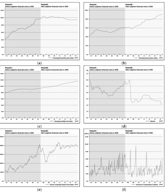
Figure 8. Market change following decreases in supply and increases in demand. 4. Empirical Analysis 4.1. Empirical Procedure In this study, the variables were selected as shown in Table 1 based on the above FDW model. That is, the housing market was divided into the transaction market, which is an asset market, and the rent market, which is a property market; and the rent market was subdivided into the chonsei and the monthly rent markets to reflect the unique characteristics of the Korean housing market. In this paper, Housing Transaction Price, Housing Chonsei Price, and Housing Monthly Rent were set as the variables that represent each market. In addition, the KOSPI was defined as the macroeconomic variable that is the first quadrant variable of the FDW model. As the KOSPI is the composite stock price index of Korea and can be used not only to check the macro market situation but also to take into account the overall flow of the investment market, it was utilized as a variable here. Next, the interest rate, which is a major variable in buying a house, was selected as an analytic variable. In the FDW model, a dynamic model is constructed in accordance with the movement of prospective buyers between the space market and the asset market. When a house is purchased, most of the funds are generally raised through a loan, as a considerable amount is required, at which time the interest rate becomes an important factor in the loan decision. For this reason, as the interest rate is presumed to have a very significant effect on prospective buyers, it was selected as an analytic variable. Finally, housing supply was selected as an analytic variable. Housing supply has a close relation with the fourth quadrant of the FDW model. The relevant data was acquired from Statistics Korea. The first analysis period was from April 2001 to December 2007 and was set as Period A and the second period from January 2008 to December 2014 was set as Period B to grasp the structural changes in the housing market before and after macroeconomic fluctuations in 2008. Figure 9 shows trend of variables before and after the subprime financial crisis.
Figure 8.Market change following decreases in supply and increases in demand.
4. Empirical Analysis
4.1. Empirical Procedure
In this study, the variables were selected as shown in Table1based on the above FDW model. That is, the housing market was divided into the transaction market, which is an asset market, and the rent market, which is a property market; and the rent market was subdivided into the chonsei and the monthly rent markets to reflect the unique characteristics of the Korean housing market. In this paper, Housing Transaction Price, Housing Chonsei Price, and Housing Monthly Rent were set as the variables that represent each market. In addition, the KOSPI was defined as the macroeconomic variable that is the first quadrant variable of the FDW model. As the KOSPI is the composite stock price index of Korea and can be used not only to check the macro market situation but also to take into account the overall flow of the investment market, it was utilized as a variable here. Next, the interest rate, which is a major variable in buying a house, was selected as an analytic variable. In the FDW model, a dynamic model is constructed in accordance with the movement of prospective buyers between the space market and the asset market. When a house is purchased, most of the funds are generally raised through a loan, as a considerable amount is required, at which time the interest rate becomes an important factor in the loan decision. For this reason, as the interest rate is presumed to have a very significant effect on prospective buyers, it was selected as an analytic variable. Finally, housing supply was selected as an analytic variable. Housing supply has a close relation with the fourth quadrant of the FDW model. The relevant data was acquired from Statistics Korea. The first analysis period was from April 2001 to December 2007 and was set as Period A and the second period
from January 2008 to December 2014 was set as Period B to grasp the structural changes in the housing market before and after macroeconomic fluctuations in 2008. Figure9shows trend of variables before and after the subprime financial crisis.Sustainability 2016, 8, 415 10 of 19
(a) (b)
(c) (d)
(e) (f)
Figure 9. Trend of variables before and after the subprime financial crisis. (a) housing transaction price index; (b) housing chonsei price index; (c) housing monthly rent index; (d) interest; (e) Korea composite stock price Index; (f) amount of construction contract.
Table 1. Variables and descriptions.
Series Descriptions Period Frequency
A B
HTI Housing transaction price index April 2001–December 2007 January2008–December2014 Monthly HJI Housing chonsei price index April 2001–December 2007 January2008–December2014 Monthly HRI Housing monthly rent index April 2001–December 2007 January2008–December2014 Monthly CDI Interest April 2001–December 2007 January2008–December2014 Monthly KOSPI Korea composite stock price index April 2001–December 2007 January2008–December2014 Monthly ACC Amount of construction contract April 2001–December 2007 January2008–December2014 Monthly
Figure 9. Trend of variables before and after the subprime financial crisis. (a) housing transaction price index; (b) housing chonsei price index; (c) housing monthly rent index; (d) interest; (e) Korea composite stock price Index; (f) amount of construction contract.
When a series analysis is conducted, the stationary series data should be ensured. If a series analysis is conducted utilizing non-stationary serial data, a spurious regression phenomenon appears where the variables look as if they have a high correlation even though there is no correlation between them [25]. To test the series data, an investigation should review whether or not a unit root exists in the serial data, and, if a unit root exists, the serial data are non-stationary. In this paper, to test the series
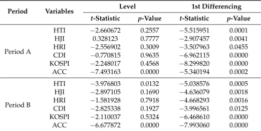
data, the ADF (augmented Dickey–Fuller) test method, which is a typical unit root test, was utilized. As in Table2below, the result of carrying out a unit root test showed that, in the null hypothesis, there was a unit root and it could not be rejected because most of the DF-t statistic values in both Periods A and B were found to be larger than the 1%, 5%, and 10% significance levels in the case of the level variables. However, the result of carrying out a unit root test by primarily differencing the level variables of both Periods A and B rejected the null hypothesis that there was a unit root at the 1%, 5%, and 10% significance levels.
Table 1.Variables and descriptions.
Series Descriptions Period Frequency
A B
HTI Housing transaction price index April 2001–December 2007 January2008–December2014 Monthly HJI Housing chonsei price index April 2001–December 2007 January2008–December2014 Monthly HRI Housing monthly rent index April 2001–December 2007 January2008–December2014 Monthly CDI Interest April 2001–December 2007 January2008–December2014 Monthly KOSPI Korea composite stock price index April 2001–December 2007 January2008–December2014 Monthly ACC Amount of construction contract April 2001–December 2007 January2008–December2014 Monthly
Table 2.Tests for unit roots (augmented Dickey–Fuller tests).
Period Variables Level 1st Differencing
t-Statistic p-Value t-Statistic p-Value
Period A HTI ´2.660672 0.2557 ´5.515951 0.0001 HJI 0.328123 0.7777 ´2.907457 0.0041 HRI ´2.556902 0.3009 ´3.507963 0.0455 CDI ´0.770815 0.9635 ´6.962115 0.0000 KOSPI ´2.248017 0.4568 ´8.299820 0.0000 ACC ´7.493163 0.0000 ´5.340194 0.0002 Period B HTI ´3.976803 0.0132 ´5.038576 0.0005 HJI ´2.897105 0.1690 ´4.636079 0.0018 HRI ´1.581928 0.7918 ´4.668293 0.0016 CDI ´2.825338 0.1927 ´3.996561 0.0125 KOSPI ´2.110037 0.5324 ´6.468610 0.0000 ACC ´6.677872 0.0000 ´7.993060 0.0000
Notes: The number of lags is selected using the Schwarz information criterion with pmax= 11.
If a co-integration relation exists between the variables even though they are of a non-stationary time series, the result of traditional regression analysis can become significant. If a co-integration exists, the analysis has to be conducted using the VECM [26].
As an error occurs when the length of the time lag is set randomly, the optimum time lag should be tested based on the information theory to ensure the reliability of the study. In general, the methods to determine the time lag p of the VAR (p) model include the AIC (Akaike information criterion) method and the SIC (Schwarz information criterion) method; the point where the value is minimized in each standard is determined as the optimum time lag. Though the explanatory power of the model is enhanced when the optimum time lag drawn through this is introduced as a new variable, the degree of freedom decreases at the same time because the size of the model grows. For this reason, a shorter time lag is selected to ensure the brevity of the model [27]. Accordingly, in this paper, the SIC reference time lag 1 was determined as the optimum time lag by testing the optimum time lag as shown in Table3below.
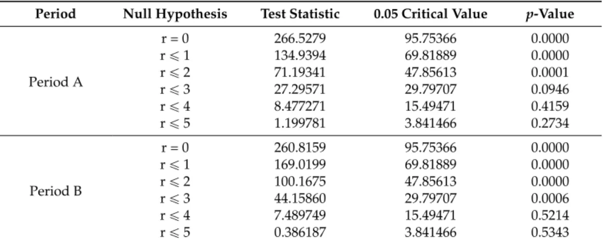
As can be confirmed in Table4below, in this paper, a co-integration relation was shown to exist at the significance level of 5% because the null hypothesis, “the number of co-integrations is smaller than
or same as r”, was rejected as a result of conducting the Johansen test, a representative co-integration test method. As it was confirmed that co-integration existed between the level variables through this, the analysis was carried out using the VECM.
Table 3.Lag specification results.
Period A Period B
Lag AIC SIC Lag AIC SIC
0 ´27.41444 ´27.22619 0 ´31.01355 ´30.82955 1 ´29.80545 ´28.48765 1 ´33.44839 ´32.16036 2 ´30.32205 ´27.87471 2 ´33.60267 ´31.21060 3 ´30.33286 ´26.75598 3 ´33.66207 ´30.16597 4 ´30.73764 ´26.03122 4 ´33.82469 ´29.22456 5 ´31.00165 ´25.16569 5 ´34.01798 ´28.31382 6 ´31.56746 ´24.60196 6 ´33.73530 ´26.92711 7 ´32.23282 ´24.13777 7 ´33.73530 ´25.67237
Table 4.Co-integration test results.
Period Null Hypothesis Test Statistic 0.05 Critical Value p-Value
Period A r = 0 266.5279 95.75366 0.0000 r ď 1 134.9394 69.81889 0.0000 r ď 2 71.19341 47.85613 0.0001 r ď 3 27.29571 29.79707 0.0946 r ď 4 8.477271 15.49471 0.4159 r ď 5 1.199781 3.841466 0.2734 Period B r = 0 260.8159 95.75366 0.0000 r ď 1 169.0199 69.81889 0.0000 r ď 2 100.1675 47.85613 0.0000 r ď 3 44.15860 29.79707 0.0006 r ď 4 7.489749 15.49471 0.5214 r ď 5 0.386187 3.841466 0.5343
Significant at 5% level; r is co-integration rank.
More specifically, the VECM for each housing market can be written as
∆HTIt“ δ ` α`β1yt´1` ρ0˘` p ÿ i“1 γ1,i∆HTIt´i` p ÿ i“1 γ2,i∆HJIt´i` p ÿ i“1 γ3,i∆HRIt´i ` p ÿ i“1 γ4,i∆CDIt´i` p ÿ i“1 γ5,i∆KOSPIt´i` p ÿ i“1 γ6,i∆ACCt´i`ut (3) ∆HJIt“ δ ` α`β1yt´1` ρ0˘` p ÿ i“1 γ1,i∆HJIt´i` p ÿ i“1 γ2,i∆HTIt´i` p ÿ i“1 γ3,i∆HRIt´i ` p ÿ i“1 γ4,i∆CDIt´i` p ÿ i“1 γ5,i∆KOSPIt´i` p ÿ i“1 γ6,i∆ACCt´i`ut (4) ∆HRIt“ δ ` α`β1yt´1` ρ0 ˘ ` p ÿ i“1 γ1,i∆HRIt´i` p ÿ i“1 γ2,i∆HTIt´i` p ÿ i“1 γ3,i∆HJIt´i ` p ÿ i“1 γ4,i∆CDIt´i` p ÿ i“1 γ5,i∆KOSPIt´i` p ÿ i“1 γ6,i∆ACCt´i`ut (5)
where α is the adjustment coefficient, β are the long-run parameters of the VEC function, and γj,ireflects the short-run aspects of the relationship between the independent variables and the target variable.
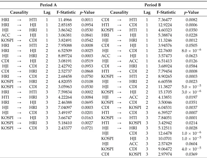
In the case of the VECM, the analysis results change sensitively and different reports are derived depending on the arrangement sequence of the endogenous variables. Therefore, the arrangement sequence of the variables according to their causality should be determined before organizing the VECM. For this, a Granger causality test was carried out here. The Granger causality test is the method used to clearly classify causal variables, and consequent variables are excluded by utilizing the lag distributed model of the state economic theories [28].
As a result of carrying out the Granger causality test during Period A, the causality was confirmed to be KOSPI > Housing supply > Chonsei price > Interest rate > Monthly rent > Transaction price, as shown in Table5. Additionally, in the case of Period B, the causality was confirmed to be KOSPI > Transaction price > Housing supply > Chonsei price > Interest rate > Monthly rent as shown in Table5. An analysis model was established by arranging the variables for Periods A and B, each based on the results of the Granger causality test.
Table 5.Results of Granger causality test.
Period A Period B
Causality Lag F-Statistic p-Value Causality Lag F-Statistic p-Value
HRI Ñ HTI 1 11.4966 0.0011 CDI Ñ HTI 1 7.36477 0.0082
HRI Ñ HJI 1 2.85185 0.0954 HTI Ñ CDI 1 12.9224 0.0006
HJI Ñ HRI 1 3.86342 0.0530 KOSPI Ñ HTI 1 4.60323 0.0350
ACC Ñ HJI 1 3.06381 0.0841 HRI Ñ HJI 1 5.38874 0.0228
KOSPI Ñ CDI 1 3.82491 0.0542 HJI Ñ HRI 1 11.3246 0.0012
HRI Ñ HTI 2 7.95088 0.0008 CDI Ñ HJI 1 3.94576 0.0505
HRI Ñ HJI 2 6.52509 0.0025 HJI Ñ CDI 1 22.7600 8.0 ˆ 10´6
HJI Ñ HRI 2 8.89724 0.0003 ACC Ñ HJI 1 3.57473 0.0623
CDI Ñ HJI 2 3.08191 0.0519 HJI Ñ ACC 1 6.51413 0.0126
HJI Ñ CDI 2 2.42792 0.0953 CDI Ñ HRI 1 3.68924 0.0584
CDI Ñ HRI 2 2.52737 0.0868 HTI Ñ CDI 2 7.79454 0.0008
HRI Ñ CDI 2 2.68458 0.0750 KOSPI Ñ HTI 2 8.90265 0.0003
KOSPI Ñ HRI 2 4.82055 0.0108 HJI Ñ HRI 2 6.60558 0.0023
KOSPI Ñ CDI 2 3.05963 0.0530 HJI Ñ CDI 2 11.3827 5.0 ˆ 10´5
HRI Ñ HTI 3 7.59834 0.0002 KOSPI Ñ HJI 2 15.1705 3.0 ˆ 10´6
HTI Ñ HRI 3 4.22264 0.0084 HJI Ñ ACC 2 4.13851 0.0197
HRI Ñ HJI 3 2.46388 0.0695 KOSPI Ñ CDI 2 3.50046 0.0351
HJI Ñ HRI 3 7.04097 0.0003 CDI Ñ KOSPI 2 6.04531 0.0037
HJI Ñ CDI 3 3.49197 0.0201 HTI Ñ CDI 3 6.39527 0.0007
KOSPI Ñ HJI 3 3.66747 0.0163 KOSPI Ñ HTI 3 7.84051 0.0001
KOSPI Ñ HRI 3 5.18410 0.0027 HTI Ñ KOSPI 3 3.42942 0.0214
KOSPI Ñ CDI 3 2.43377 0.0721 HJI Ñ HRI 3 5.12511 0.0028
HJI CDI 3 12.6478 1.0 ˆ 10´6 KOSPI HJI 3 10.0701 1.0 ˆ 10´5 HJI ACC 3 2.57429 0.0604 KOSPI CDI 3 9.06472 4.0 ˆ 10´5 CDI KOSPI 3 2.97974 0.0369 4.2. Results
An impulse response analysis analyzes the correlation between variables and the ripple effect by applying an impact of standard deviation 1 to a variable and examining the changes in the variable and in other variables for a certain period of time. In this paper, the structure of the Korean housing market as it went through rapid macroeconomic fluctuations pre- and post-2008 was comparatively analyzed through an impulse response analysis.
We first look at Period A as shown in Figure10a. Here, the transaction price changes in a positive (+) direction through the impulse of the chonsei price, and this change is shown to be the biggest.
Additionally, the transaction price changes in a positive (+) direction through the impulses of the monthly rent, KOSPI, and housing supply. Though the transaction price changes in a negative (´) direction through the impulse of the interest rate at the beginning of the period, the change converts toa positive (+) direction over time. As shown in Figure10b, the chonsei price changes in a positive (+) direction through the impulse of the chonsei price itself, showing the biggest fluctuation, and also changes in a positive (+) direction through the impulses of the housing supply and the interest rate. The chonsei price changes in a negative (´) direction through the impulses of the transaction price and monthly rent. Figure10c shows the change in the monthly rent for the impulse of each variable. The monthly rent changes in a positive (+) direction through the impulses of the housing supply and interest rate. In addition, though it changes in a negative (´) direction through the impulses of KOSPI and the chonsei price at the beginning of the period, the change converts to a positive (+) direction over time. Finally, the monthly rent changes in a negative (´) direction through the impulse of the transaction price.
Sustainability 2016, 8, 415 14 of 19 changes in a positive (+) direction through the impulse of the chonsei price itself, showing the biggest fluctuation, and also changes in a positive (+) direction through the impulses of the housing supply and the interest rate. The chonsei price changes in a negative (−) direction through the impulses of the transaction price and monthly rent. Figure 10c shows the change in the monthly rent for the impulse of each variable. The monthly rent changes in a positive (+) direction through the impulses of the housing supply and interest rate. In addition, though it changes in a negative (−) direction through the impulses of KOSPI and the chonsei price at the beginning of the period, the change converts to a positive (+) direction over time. Finally, the monthly rent changes in a negative (−) direction through the impulse of the transaction price. (a) (b) (c) (d) (e) (f) Figure 10. Impulse response graph. (a) impulse response of HTI—Period A; (b) impulse response of HJI—Period A; (c) impulse response of HRI—Period A; (d) impulse response of HTI—Period B; (e) impulse response of HJI—Period B; (f) impulse response of HRI—Period B.
Next, looking at Period B as shown in Figure 10d, the transaction price changes in a positive (+) direction through the impulse of the transaction price itself, showing the biggest fluctuation. In addition, the transaction price changes in a positive (+) direction through the impulses of KOSPI Figure 10. Impulse response graph. (a) impulse response of HTI—Period A; (b) impulse response of HJI—Period A; (c) impulse response of HRI—Period A; (d) impulse response of HTI—Period B; (e) impulse response of HJI—Period B; (f) impulse response of HRI—Period B.
Next, looking at Period B as shown in Figure10d, the transaction price changes in a positive (+) direction through the impulse of the transaction price itself, showing the biggest fluctuation. In addition, the transaction price changes in a positive (+) direction through the impulses of KOSPI and the chonsei price. It changes in a negative (´) direction through the impulse of the housing supply and does not show hardly any change for the impulses of the interest rate and the monthly rent. As shown in Figure10e, the chonsei price changes in a negative (´) direction through the impulse of the housing supply, showing the biggest fluctuation. Additionally, it is confirmed that the chonsei price is affected by the impulses of the chonsei price itself and of the transaction price and KOSPI changing in a positive (+) direction. As shown in Figure10f, the monthly rent changes in a negative (´) direction through the impulse of housing supply, showing the biggest fluctuation. In addition, the monthly rent is confirmed to be affected by the impulses of the KOSPI, the transaction price, and the chonsei price changing in a positive (+) direction and by the impulse of the interest rate changing in a negative (´) direction.
Tables6–8presents the significant implications derived from comparatively analyzing the results of the impulse responses for Periods A and B.
Table 6.Comparison of the impulse response (IR) of housing transaction market.
Results Implications
- As can be seen from Figure10a,d, the impulse of the transaction price shows a positive (+) relation with the transaction price itself.
- During an economic invigoration period, an increase in the transaction price generates continuous demand by raising expectations for an increase in the housing transaction price. - However, during an economic depression, a decrease in the
housing transaction price has an effect on the continuous drop in housing prices by raising concerns over further decreases in housing transaction prices.
- When Figure10a,d are compared, though the fluctuation decreases over time, it is confirmed that the fluctuation caused by the transaction price itself during Period A is bigger than that of Period B.
- During an economic depression period, as the expectations for an increase in housing prices in Korea are relatively low, the investment demand weakens.
- The transaction price changes in a positive (+) direction by the impulse of the chonsei price in Figure10a, and, though the transaction price changes in a positive (+) direction by the impulse of chonsei price in Figure10d, the fluctuation is relatively small.
- During an economic invigoration period, the increase in space demand is naturally converted to the housing transaction market. - During an economic depression period, the increase in the chonsei
price also has an effect on the increase in the transaction price. However, the effect is much smaller than during an economic invigoration period. This is thought to be because the overall market depression, that is, the macroeconomic environment, has a much bigger effect on the change in the housing transaction price than the supply/demand condition of the chonsei market.
- The transaction price changes in a positive (+) direction by the impulse of monthly rent in Figure10a. Though the transaction price changes in a negative (´) direction by the impulse of monthly rent in Figure10d, the fluctuation is very small.
- During an economic invigoration period, the monthly rent market is invigorated as a new space demand is generated, and a new investment demand is generated in expectation of this. - During an economic depression period, the housing transaction
price is shown to drop even when the monthly rent increases. This is thought to be because there is the chonsei market in Korea. If the deposit funds can be arranged, the chonsei, which does not involve any monthly rent, is most advantageous to space demander. The reason why the monthly rent increases nonethelessis because more demand moves from the chonsei market to the monthly rent market than to the transaction market. Moreover, the reason why the monthly rent market impulse on the fluctuation of the transaction price is very small is thought to be because the effect is relatively weakened as the chonsei supply is converted to the monthly rent supply.
Table 7.Comparison of the impulse response (IR) of housing chonsei market.
Results Implications
- While the impulse of the transaction price and the change in chonsei price show a negative (´) relation in Figure10b, they show a positive (+) relation in Figure10e.
- During an economic invigoration period, the expectations for an increase in housing transaction prices are high. Accordingly, not only investment demand but also space demand flows into the transaction market. After all, the impulse of the transaction price shows a negative (´) relation with the change in the housing chonsei price.
- During an economic depression period, the space demand in the chonsei market does not move to the transaction market but prefers the chonsei market. The reason why the impulse of the transaction market and the change in the chonsei price show a positive (+) relation nonetheless is thought to be because space demand in the chonsei market moves to the monthly rent market.
- Though the impulse of monthly rent and the change in the chonsei price show a negative (´) relation in Figure10b, e, the fluctuation is small.
- Between the monthly rent market and the chonsei market, space demanders prefer the chonsei market where no monthly rent is paid. As can be confirmed in the Granger causality test results above, between the chonsei market and the monthly rent market, which are both rent markets, as the monthly rentmarket follows the movement of the chonsei market, though the change in the chonsei price and the impulse of the monthly rent show a negative (´) relation, the effect is thought to be very small.
Table 8.Comparison of the impulse response (IR) of housing monthly rent market.
Results Implications
- Though the monthly rent shows a negative (´) relation with the impulse of chonsei price at the beginning of the period in Figure10c, it gradually converts to a positive (+) relation over time. However, it shows a positive (+) relation from the beginning in Figure10f.
- The space demanders in the chonsei and monthly rent markets enter other markets due to diverse reasons such as price increases in the relevant marketsand changes in household income. In such cases, during an economic invigoration period, an increase in the chonsei price means that new demand for chonsei is generated, and as new demand for chonsei may be converted from demand for monthly rentals, it may have a negative (´) relation. However, the reason why the relevant relation converts to a positive (+) direction is because the demanders of chonsei, who cannot afford the increase in the chonsei price, move again to the monthly rental market.
- However, during an economic depression period, the monthly rent response following the change in the chonsei price is faster than during an economic invigoration period. That is, many of the demanders of chonsei are unable to deal with the increase in the deposit amount as the imbalance between the demand and supply was very severe after the financial crisis.
- While the impulse of the transaction price shows a negative (´) effect on the monthly rent in Figure10c, it has a positive (+) effect in Figure10f.
- During an economic invigoration period, as the space demanders are concentrating on the transaction market, an increase in the transaction price is thought to have an effect on the rent market. - During an economic depression period, as it is difficult to expect
an investment profit in the transaction market, the rental quantity supplied to the chonsei market is converted to the monthly rent market. For this reason, monthly rents drop.
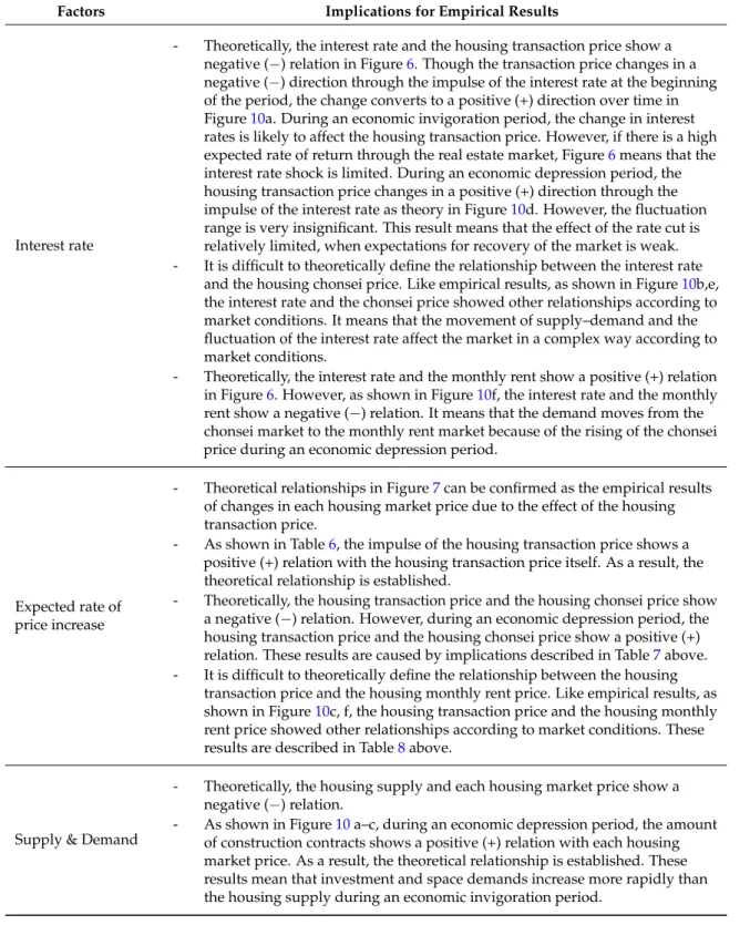
Table9explains about the connections between the theoretical framework and empirical results. Table 9.The connections between the theoretical framework and empirical results.
Factors Implications for Empirical Results
Interest rate
- Theoretically, the interest rate and the housing transaction price show a negative (´) relation in Figure6. Though the transaction price changes in a negative (´) direction through the impulse of the interest rate at the beginning of the period, the change converts to a positive (+) direction over time in Figure10a. During an economic invigoration period, the change in interest rates is likely to affect the housing transaction price. However, if there is a high expected rate of return through the real estate market, Figure6means that the interest rate shock is limited. During an economic depression period, the housing transaction price changes in a positive (+) direction through the impulse of the interest rate as theory in Figure10d. However, the fluctuation range is very insignificant. This result means that the effect of the rate cut is relatively limited, when expectations for recovery of the market is weak. - It is difficult to theoretically define the relationship between the interest rate
and the housing chonsei price. Like empirical results, as shown in Figure10b,e, the interest rate and the chonsei price showed other relationships according to market conditions. It means that the movement of supply–demand and the fluctuation of the interest rate affect the market in a complex way according to market conditions.
- Theoretically, the interest rate and the monthly rent show a positive (+) relation in Figure6. However, as shown in Figure10f, the interest rate and the monthly rent show a negative (´) relation. It means that the demand moves from the chonsei market to the monthly rent market because of the rising of the chonsei price during an economic depression period.
Expected rate of price increase
- Theoretical relationships in Figure7can be confirmed as the empirical results of changes in each housing market price due to the effect of the housing transaction price.
- As shown in Table6, the impulse of the housing transaction price shows a positive (+) relation with the housing transaction price itself. As a result, the theoretical relationship is established.
- Theoretically, the housing transaction price and the housing chonsei price show a negative (´) relation. However, during an economic depression period, the housing transaction price and the housing chonsei price show a positive (+) relation. These results are caused by implications described in Table7above. - It is difficult to theoretically define the relationship between the housing
transaction price and the housing monthly rent price. Like empirical results, as shown in Figure10c, f, the housing transaction price and the housing monthly rent price showed other relationships according to market conditions. These results are described in Table8above.
Supply & Demand
- Theoretically, the housing supply and each housing market price show a negative (´) relation.
- As shown in Figure10a–c, during an economic depression period, the amount of construction contracts shows a positive (+) relation with each housing market price. As a result, the theoretical relationship is established. These results mean that investment and space demands increase more rapidly than the housing supply during an economic invigoration period.
5. Conclusions
The objective of this paper is to comparatively analyze the dynamic relationship between the Korean housing transaction market, chonsei housing market, and housing monthly rent market before and after macroeconomic fluctuations. This is done by defining the Korean housing market utilizing the FDW model and setting the analytical variables accordingly. Through this, we derive implications