A Combustion Instability Analysis of a Model Gas Turbine Combustor by the Transfer Matrix Method

A Combustion Instability Analysis of a Model Gas Turbine Combustor by

the Transfer Matrix Method

Dong Jin Cha

†

· Jay H. Kim

*

· Yong Jin Joo

**

Key Words : Combustion instability, model gas turbine combustor, normal mode method, stability margin

thermoacoustics, transfer matrix method

Abstract

Combustion instability is a major issue in design of gas turbine combustors for efficient operation with low emissions. Combustion instability is induced by the interaction of the unsteady heat release of the combustion process and the change in the acoustic pressure in the combustion chamber. In an effort to develop a technique to predict self-excited combustion instability of gas turbine combustors, a new stability analysis method based on the transfer matrix method is developed. The method views the combustion system as a one-dimensional acoustic system with a side branch and describes the heat source as the input to the system. This approach makes it possible to use the advantages of not only the transfer matrix method but also well-established classic control theories. The approach is applied to a simple gas turbine combustion system to demonstrate the validity and effectiveness of the approach.

1. Introduction

Combustion instability is induced by the coupling effect of the unsteady heat release of the combustion process and the change in the acoustic pressure in the gas manifold of the combustion chamber [1,2,3]. Such instabilities can cause various problems in the combustion system, including poor efficiency, premature degradation of components, and even a catastrophic failure of the system. Because the combustion instability is a very complex phenomenon, an accurate, full-scale quantitative analysis of the non-linear combustion response is very difficult. However, a simple but reliable analysis method can be developed to predict the onset of combustion instability based on a linear model. Such a method can be used to understand the condition of the instability and to obtain design guidelines.

The main purpose of this paper was to develop a new approach based on the transfer matrix method to analyze the combustion instability. The transfer matrix, which is also called four-pole matrix, is a very convenient concept to model a complex one-dimensional acoustic systems [4,5]. Richards et al. applied the transfer matrix method to model the combustion system as a feed-back control system [3]. In their model, the transfer matrix method was used to obtain impedances at various points, which were used to obtain the control model. The method we

developed in this paper, the combustion system is modeled by using a side branch description to represent the flame point as the system input. This enables much simpler, straightforward modeling of the system.

2. Description of the System by a Wave Eq.

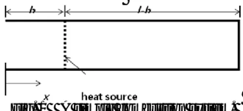
Figure 1 shows a simple combustion system that will be used to develop the analysis method. A large plenum is attached to the left end, which is modeled as the pressure release end, and the flow is restricted in the right end, which is modeled as the close end. The heat source at x=b is modeled as a point source. The combustion process is described by:

(1)

where, p is the acoustic pressure, c is the sonic velocity and hw is the source term due to combustion. For the 1-D system shown in Fig. 1, the equation becomes [2]

(2) where, q is the rate of heat release per area and is the Dirac delta function. A model that relates the heat release and acoustic variables is necessary. One of simple models is

Fig. 1 A simple combustion system.

† Department of Building Services Engineering, Hanbat National University, Daejeon Korea

E-mail : djcha@hanbat.ac.kr

TEL:+82-42-821-1182 FAX:+82-42-821-1175

* Department of Mechanical Engineering, The University of Cincinnati, Cincinnati, Ohio, U.S.A

** IGCC Group, Korea Electric Power Research Institute, Daejeon Korea w h p t p c     2 2 2 2 1 ) ( 1 1 2 2 2 2 2 2 x b t q c x p t p c            _ ) (xb  대한기계학회 2008년도 추계학술대회 논문집

(3) where, u(b-, t-τ) is the particle velocity at x = b-, τ is the time delay, which is the convection time from fuel injection to its combustion, and β is a non-dimensional parameter that has to be determined empirically.

Eq. (2) can be compared with the Lighthill’s equation, an inhomogeneous wave equation with a mass flow source.

(4) where, mis the mass flow input to the system per unit volume. By comparing Eq. (4) with Eq. (2), we find that

(5) Substituting Eq. (3) into Eq. (5) and simplifying, we find that

(6) If the flow is harmonic, etc, Eq. (6) becomes

(7) where, upper case implies the harmonic amplitude.

3. Review of Two Existing Solution Methods

3.1 Method Based on Assumed Modeshape

In the system shown in Fig. (1), the boundary conditions are

(8) The conditions are satisfied if P(x)=Asin(kx) and P(x)= Bcos[k(l-x)], respectively. With these, at x=b, the pressure continuity condition is

(9) The velocity jump condition is

(10) Combining Eqs. (9) and (10), the frequency equation is obtaind as

(11) The resonance frequency can be obtained by solving Eq. (11) by a numerical method. If the ith root of Eq. (11) is, ωi the normalized frequency and normalized growth rate are obtained as

(12) (13) where ωni is the ith undamped resonant frequency. A positive growth rate gNi indicates that the combustion unstable.

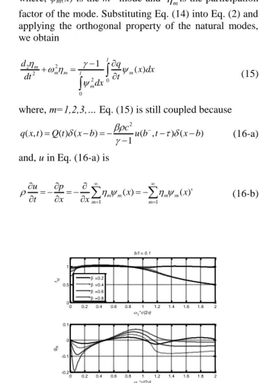
Figure 2 shows the trend of instability as a function of the growth rate β and the time delay τ. Notice that the combustion process becomes unstable in the frequency range in that gN is positive. The magnitude of gN indicates the strength of instability.

3.2 Solution by Galerkin’s Method

The pressure in the system can be assumed as a linear superposition of the natural modes as follows.

(14) where, ψm(x) is the mth mode and



mis the participation factor of the mode. Substituting Eq. (14) into Eq. (2) and applying the orthogonal property of the natural modes, we obtain

(15)

where, m=1,2,3,… Eq. (15) is still coupled because (16-a) and, u in Eq. (16-a) is

(16-b)

Fig. 2 Variation of instability frequency and growth

rate with τ for the root of Eq. (11) near 𝜔_𝑛𝑖, taking b/l = 0.1 and β’s different [Similar to one in Ref. 2].

0 0.2 0.4 0.6 0.8 1 1.2 1.4 1.6 1.8 2 0 0.5 1 1*/(2) fN b/l = 0.1  =0.2  =0.4  =0.6  =0.8 0 0.2 0.4 0.6 0.8 1 1.2 1.4 1.6 1.8 2 -0.2 -0.1 0 0.1 1*/(2) gN ) , ( 1 ) ( 2    _     t b u c t q t m x p t p c         ( ) 1 2 2 2 2 2 



( , ) ( , )



) ( ) ( 1 2 Qt mt u ub t ub t c s   _     _{ }   ) , ( ) , ( ) , (bt ubt ubt u ) 1 )( ( ) (  j e b U b U      , 0 ) 0 (  P U(l)0 )] ( cos[ ) sin(kb B k l b A   ) 1 )( cos( )] ( sin[  j e kb A b l k B       j e b l k kb)tan[ (  )]1  tan( ni i Ni f  ) Re(  ni i Ni g  ) Im(  





     l l m m m m m _xdx t q dx dt d 0 0 2 2 2 2 1  _{( )}      ) ( ) , ( 1 ) ( ) ( ) , ( 2 b x t b u c b x t Q t x q         _{ }   







               1 1 )' ( ) ( m m m m m m x x x x p t u _{ } 



   1 ) ( ) ( ) , ( m m mt x t x p  

(a) ω1τ/(2π)=0.0

(b) ω1τ/(2π)=1.2

(c) ω1τ/(2π)=1.8

(d) ω1τ/(2π)=2.0

Fig. 3 Variation of disturbance in combustion dynamic

pressure with β of 0.2 and different values of ω1τ/(2π) shown in Fig. 2.

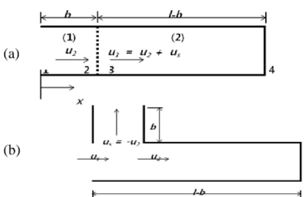
Fig. 4 Combustor modeled as a 1-D duct. (a) 1-D duct

model and (b) 1-D duct model with a side branch description.

Culick suggested a simplification of Eq. (15) by keeping only the fundamental mode (m=1) in evaluating Eq. (16-a) [1]. Figure 3 shows η1 and dη1/dtobtained as such, which are the time histories of combustion dynamic pressure with several different values of τ while β is fixed at 0.2. Figure 3(a), which is for τ=0, shows the disturbance remains constant. In Figs. 3(b) where gN is negative, the disturbance decays. In Figs. 3(c) and (d), where gN is positive, the disturbance grows, latter case growing more slowly. These observations are compatible with what we observed in Fig. 2.

4. Transfer Matrix Based Method

The transfer matrix method, also known as four pole method, is an ideal method to analyze a combustor system composed of sections of various different cross-sectional area and side-branches [6]. In this work, we developed a new approach to apply the transfer matrix method more easily to combustion system analysis. The approach rearranges the system model to make the heat source point the input point of the system by viewing a part of the combustion duct as a side-branch. It is shown that the method is completely equivalent with the other methods as long as they used the same heat source model.

Figure 4 shows the 1-D system in Fig. 1 represented as a combination of two sub-elements. Figure 4(a) shows a typical model and Fig. 4(b) shows the system with the left end of the duct described as a side branch. Model in Fig. 4(b) enables the volume flow input us due to the heat release to be described as the system input. In the system shown in Fig. 4(a), the boundary conditions are given as

(17) It is more convenient to use acoustic mass flow velocity than the particle velocity in formulation of the transfer matrix of the combustion duct because the cross-sectional area and temperature change throughout the system. For the ith section of the duct, we define

0 0.02 0.04 0.06 0.08 0.1 0.12 0.14 0.16 0.18 0.2 -1 -0.5 0 0.5 1 Time (s)  1 ₁/(2) = 0,0 0 0.02 0.04 0.06 0.08 0.1 0.12 0.14 0.16 0.18 0.2 -1000 -500 0 500 1000 Time (s) d  1 /d t 0 0.02 0.04 0.06 0.08 0.1 0.12 0.14 0.16 0.18 0.2 -1 -0.5 0 0.5 1 Time (s)  1 1/(2) = 1.2 0 0.02 0.04 0.06 0.08 0.1 0.12 0.14 0.16 0.18 0.2 -1000 -500 0 500 1000 Time (s) d  1 /d t 0 0.02 0.04 0.06 0.08 0.1 0.12 0.14 0.16 0.18 0.2 -20 -10 0 10 20 Time (s)  1 1/(2) = 1.8 0 0.02 0.04 0.06 0.08 0.1 0.12 0.14 0.16 0.18 0.2 -2 -1 0 1 2x 10 4 Time (s) d  1 /d t 0 0.02 0.04 0.06 0.08 0.1 0.12 0.14 0.16 0.18 0.2 -2 -1 0 1 2 Time (s)  1 1/(2) = 2.0 0 0.02 0.04 0.06 0.08 0.1 0.12 0.14 0.16 0.18 0.2 -2000 -1000 0 1000 2000 Time (s) d  1 /d t (b) (a) , 0 1 p u40

(18) where, Vi and Ui are harmonic amplitudes of the mass flow velocity and the particle velocity, ρi and Si are the density and cross-sectional area of the ith section of the duct.

The transfer matrix equation of the system shown in Fig. 4(b) is given by [4,5]                                              0 1 1 0 1 4 4 2 2 2 2 2 2 4 4 2 2 2 2 2 V P D Z B C Z A B A U P D C B A Z V P S S S S (19) where, A2, B2, C2 and D2 are the four-pole parameters of the duct 2 of length l-b in Fig. 4(a) and Zs is the

impedance of the side branch defined as

(20) From Eq. (19), (21) (22) Therefore, (23) and, (24-a)

In terms of particle velocities,

(24-b)

Because Q (see Eq. (5)),

(25)

where is the transfer function between Us and Q. The transfer function H2 between Q and Us is

(26)

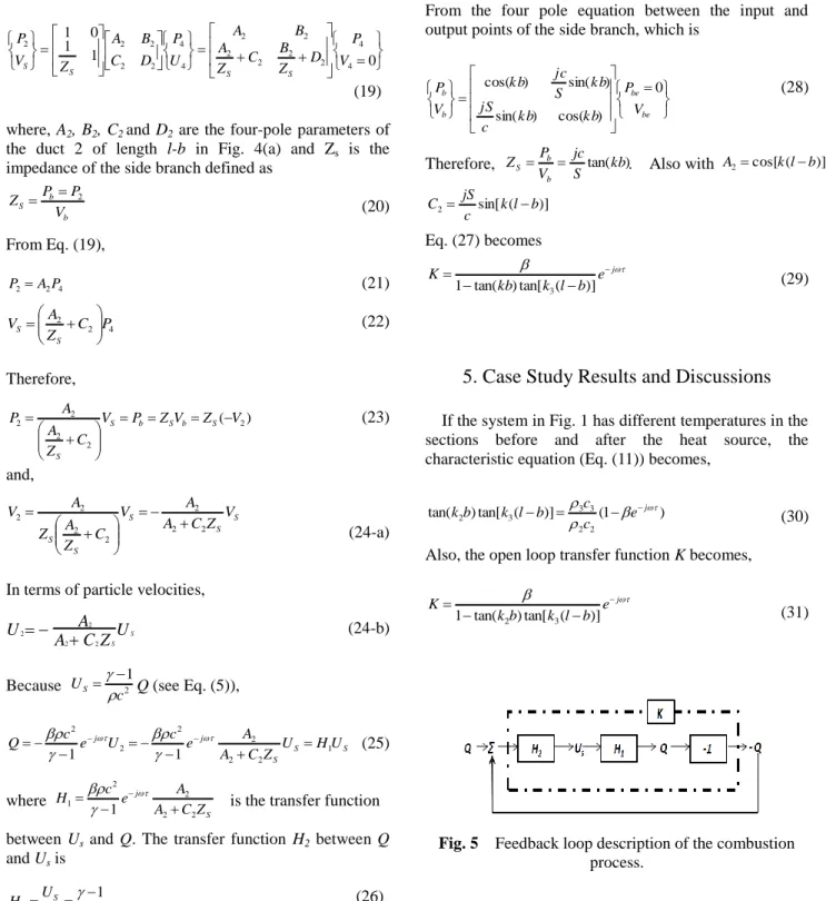
Figure 5 shows the description of the combustion system as a feedback loop. Notice that -1 is multiplied to Q to make a negative feedback loop to adopt the standard convention in control theory. From the figure, the open loop transfer function K is obtained as

(27) From the four pole equation between the input and output points of the side branch, which is

(28)

Therefore, . Also with

Eq. (27) becomes

(29)

5. Case Study Results and Discussions

If the system in Fig. 1 has different temperatures in the sections before and after the heat source, the characteristic equation (Eq. (11)) becomes,

(30) Also, the open loop transfer function K becomes,

(31)

Fig. 5 Feedback loop description of the combustion

process. S j Z C A A e c H 2 2 2 2 1 1       2 2 1 c Q U H S     2 1 c US _   i i i i SU V  b b S V P P Z   2 4 2 2 AP P  4 2 2 _{C P} Z A V S S         ) ( 2 2 2 2 2 V P ZV Z V C Z A A P S b S b S S             S S S S S V Z C A A V C Z A Z A V 2 2 2 2 2 2 2  _         U Z C A A U S S 2 2 2 2  S S S j j U H U Z C A A e c U e c Q 1 2 2 2 2 2 2 1 1              2 2 2 2 2 2 1 1 1 A CZ c A e c H H K S j                                      be be b b V P k b k b c jS k b S jc k b V P 0 ) cos( ) sin( ) sin( ) cos( ) tan(kb S jc V P Z b b S     j e b l k kb K     )] ( tan[ ) tan( 1 3 ) 1 ( )] ( tan[ ) tan( 2 2 3 3 3 2     j e c c b l k b k       j e b l k b k K     )] ( tan[ ) tan( 1 2 3 )], ( cos[ 2 k l b A   )] ( sin[ 2 kl b c jS C  

Table 1 Simulation parameters of a case studied [3]. Parameter Value (1)1) (2)1) Diameter, m 0.13335 0.13335 Length (b & (ℓ-b)), m 0.01270 1.39700 Cross-sectional area, m2 0.013966 0.013966 Temperature, K 553.3 1811.1 Pressure, MPa 2.020 2.020 Density, kg/m3 13.21 3.89 Ratio of specific heats 1.4 1.3

Mol. wt., kg/kg-mole 29.0 29.0 Sonic vel., m/s 462.7 821.6 Mean flow vel., m/s 7.64 25.93

Mach no. 0.01651 0.03156 Mass flow rate, kg/s 1.409 1.409

1)

In Fig. 4(a)

In general, a gas turbine combustion system can be modeled as a network of fuel injector including air and fuel supplies, flame, combustion chamber, exhaust nozzle, etc [3]. Table 1 lists the parameters provided used for simulations. All parameters, both geometrical and operational, are selected to be representative of gas turbine combustors which are summarized in Table 1.

(a) 1st undamped mode

(b) 2nd undamped mode

Fig. 6 Variation of instability frequency and growth

rate with τ for the root of Eq. (30) near the first two undamped frequencies among ten studied.

Table 2 Combustion instability with traditional method.

fN1,2) ω, Hz A stable case (gN<0) 2) An unstable case (gN>0) 2) ω1τ/(2π) τ , ms ω1τ/(2π) τ , ms 1.7468 143.24 0.15 1.83 0.5 6.09 1.7470 429.76 0.1 0.41 0.5 2.03 1.0482 429.76 - - - - 1.2480 716.35 0.1 0.17 0.7 1.22 1.3592 1003.09 0.1 0.14 0.7 0.95 1.1121 1003.11 - - - - 1.2102 1290.07 - - - - 1.0488 1290.02 0.1 0.08 0.85 0.69 1.1313 1578.16 - - - - 1.0122 1578.02 0.1 0.06 0.9 0.58 1)

In the first case of gN=0

2)

For β=0.2

Figure 6 shows a part of the simulation result. The figure shows that the oscillation grows or decays depending on the fixed heat input, i.e., β and the time delay τ near the 1st two undamped frequencies. For τ =0 (not reported here) the rate of heat input only shifts the frequency of oscillation.

Table 2 summarizes the simulation results which include those shown in Fig. 6. The data in the first two columns were obtained for the undamped case, gN =0. The next two columns show values of ω1τ/(2π) and τ for the stable case, i.e., gN <0. The last two columns are for the unstable cases.

Once the combustion process is represented by a control system, well established tools such as the Nyquist plot, Bode plot or root-locus method can be used for stability analysis or design of the system. Most control systems behave in a pattern such that they become unstable if the gain increases over a certain value. For these systems, in addition to determining their absolute stability, the Nyquist plot provides qualitative information as to the degree of stability. If the system is stable, the corresponding Nyquist curve does not encircle the (-1,0) point. If the system is marginally stable, the curve passes through the point. If the system is unstable, the plot encircles the point. For a stable system, the closer the Nyquist curve approaches the (-1,0) point, the less stable the system is [7].

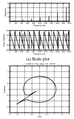
Figure 7 shows the Bode and Nyqusit plots obtained for the case we studied. The first one is the Bode plot of the open loop transfer function, which can provide the resonant frequencies of the model combustion system. Peak amplitudes in Fig. 7(a) correspond to the resonant frequencies of the system, which are listed in Table 3. As seen in the table, predicted resonant frequencies with this method agree well with those with the traditional system resonant frequency approach.

Next, Nyquist plots are used to see whether the system becomes stable or not at the stable conditions. Figure 7(b) is a Nyquist plot of an unstable case of the 1st mode (ω =143.24 Hz and τ=6.09 ms) which encircles (-1,0) point,

0 0.2 0.4 0.6 0.8 1 1.2 1.4 1.6 1.8 2 0.5 1 1.5 2 ₁*/(2) fN 1 = 515.576 rad/s (82.0565 Hz) b/l = 0.009009 T. ratio = 3.396 0 0.2 0.4 0.6 0.8 1 1.2 1.4 1.6 1.8 2 -0.2 -0.1 0 0.1 ₁*/(2) gN  =0.2  =0.4  =0.6  =0.8 0.5 0.6 0.7 0.8 0.9 1 1.1 1.2 1.4 1.6 1.8 ₁*/(2) fN 2 = 1546.7279 rad/s (246.1694 Hz) b/l = 0.009009 T. ratio = 3.396 0 0.2 0.4 0.6 0.8 1 1.2 1.4 1.6 1.8 2 -0.2 -0.1 0 0.1 ₁*/(2) gN  =0.2  =0.4  =0.6  =0.8

(a) Bode plot

(b) Nyquist plot of an unstable case at the 1st mode

(c) Nyquist plot of a stable case at the 1st mode

Fig. 7 The open loop transfer function K of a model

combustion system studied.

Table 3 Comparison of resonant frequencies with the

two methods.

implying that the system is unstable. The case in Fig. 7(c) does not encircle the (-1,0) point; therefore stable. Table 3 compares six resonant frequencies, which shows the

equivalence of the methods.

6. Conclusions

Two existing combustion instability analysis methods, the method based on the assumed modeshape method and Galerkin’s method, have been reviewed. A new method based on the transfer matrix method was developed in this work. The new approach employs a side-branch description, which enables to model the heat source point as the input point of the system. A system model that describes the combustion process as a feed-back control system can be obtained by the transfer matrix method. The approach enables exploiting all the advantages of the transfer matrix method and techniques used in the classic control theory. Transfer matrix method makes it possible to formulate the model of a combustion system of any complexity as easily as the simplest system.

Acknowledgement

This work was supported by the New & Renewable Energy Center / Korea Energy Management Corporation through the “Design and Construction of 300 MW IGCC Demonstration Plant in Korea” project funded by the Korean Ministry of Knowledge Economy.

References

(1) Culick, F. E. C., 1989, “Combustion Instabilities in Liquid-fueled Propulsion System – An Overview,” AGARD Conference Proceedings, No. 450.

(2) Dowling, P. E. and Stow, S. R., 2003, “Acoustic Analysis of Gas Turbine Combustor,” J. of Propulsion and Power, Vol. 19, No. 5, pp. 751-764. (3) Richards, G. A., Straub, D. L. and Robey, E. H.,

2003, “Passive Control of Combustion Dynamics in Stationary Gas Turbines,” J. of Propulsion and Power, Vol. 19, No. 5, pp. 795-810.

(4) Munjal, M. L., 1987, Acoustics of Ducts and Mufflers, Wiley, New York, pp. 121-130.

(5) Kim, J. and Soedel, W., 1990, “Development of General Procedure to Formulate Four Pole Parameters by Modal Expansion and Its Application to Three Dimensional Cavities,” ASME Trans. J. of Vibration and Acoustics, Vol. 112, pp. 452-459. (6) Kadam, P. and Kim, J., 2007, “Experimental

Formulation of Three-Dimensional Cavities,” J. of Sound and Vibration, Vol. 307, pp. 578-590. (7) Phillips, C. L. and Harbor, R. D., 2000, Feedback

Control System, 4th ed., Prentice-Hall, Upper Saddle River, NJ. 0 200 400 600 800 1000 1200 1400 1600 1800 2000 0 10 20 30 40 Frequency (Hz) M a g n it u d e 0 200 400 600 800 1000 1200 1400 1600 1800 2000 -200 -100 0 100 200 Frequency (Hz) P h a s e ( d e g re e s ) -2 -1.5 -1 -0.5 0 0.5 1 1.5 2 -2 -1.5 -1 -0.5 0 0.5 1 1.5 2 Real Im a g in a ry  = 6.098 ms Freq. range = 40 - 240 Hz -2 -1.5 -1 -0.5 0 0.5 1 1.5 2 -2 -1.5 -1 -0.5 0 0.5 1 1.5 2 Real Im a g in a ry No. ω, Hz w/ traditional method w/ feedback

control concept Diff. (%)

1 143 142 1 (0.70) 2 430 428 2 (0.47) 3 716 713 3 (0.42) 4 1003 998 5 (0.50) 5 1290 1284 6 (0.47) 6 1578 1570 8 (0.51)