저작자표시-비영리-변경금지 2.0 대한민국 이용자는 아래의 조건을 따르는 경우에 한하여 자유롭게 l 이 저작물을 복제, 배포, 전송, 전시, 공연 및 방송할 수 있습니다. 다음과 같은 조건을 따라야 합니다: l 귀하는, 이 저작물의 재이용이나 배포의 경우, 이 저작물에 적용된 이용허락조건 을 명확하게 나타내어야 합니다. l 저작권자로부터 별도의 허가를 받으면 이러한 조건들은 적용되지 않습니다. 저작권법에 따른 이용자의 권리는 위의 내용에 의하여 영향을 받지 않습니다. 이것은 이용허락규약(Legal Code)을 이해하기 쉽게 요약한 것입니다. Disclaimer 저작자표시. 귀하는 원저작자를 표시하여야 합니다. 비영리. 귀하는 이 저작물을 영리 목적으로 이용할 수 없습니다. 변경금지. 귀하는 이 저작물을 개작, 변형 또는 가공할 수 없습니다.
Master
’s Thesis of Landscape Architecture
A multi-layer model for
transpiration of urban tree
considering vertical structure
수직적 구조를 고려한 도시 수목의
증산량 산정 다층 모델
August 2020
Graduate School of Seoul National University
Department of Landscape Architecture and Rural
Systems Engineering, Landscape Architecture Major
A multi-layer model for
transpiration of urban tree
considering vertical structure
Under the Direction of Adviser, Prof. Dong Kun Lee
Submitting a master
’s thesis of Landscape
Architecture
July 2020
Graduate School of Seoul National University
Department of Landscape Architecture and Rural
Systems Engineering, Landscape Architecture Major
Seok Hwan Yun
Confirming the master
’s thesis written by
Seok Hwan Yun
July 2020
Chair
(Seal)
Vice Chair (Seal)
Examiner (Seal)
i
Abstract
As the urban heat island has been intensified, the cooling effect of urban trees is becoming important. Tree can reduce the radiant heat reaching the surface of the urban area by blocking or reflecting the radiant heat. In addition, the surface temperature of the tree is lower than that of the impervious surface such as asphalt and concrete, resulting in lower longwave radiation. Transpiration of tree also have cooling effect by releasing water into the atmosphere through the stomata of leaves, which reduces urban sensible heat by increasing latent heat. However, most previous studies which have conducted to calculate the transpiration rate have not focused on urban trees or oversimplified plant physiological process.
I propose a multi-layer model for transpiration of urban tree accounting for plant physiological process considering the vertical structure of trees and buildings. It is expanded from urban canopy model to simulate photosynthetically active radiation and leaf surface temperature accurately. To evaluate how building and tree conditions affect transpiration, I simulate transpiration by scenarios varying conditions of building height, tree location and vertical leaf area variation of trees. Simulations are conducted on four LAD distribution of trees; (1) Constant Density (C.D), (2) High Density, few layers (H.D), (3) High Density in Middle layers (M.H.D), (4) High Density in lower layers (L.H.D). LAI and tree height is same in all cases. The scenarios include three types of surrounding building (12m, 24m, and 36m) and two types of tree location (South and North). One of the
ii
day that was a clear day, did not have rain back and forth, had high air temperature, low relative humidity is selected (1 August 2018) in Seoul (126.9658, 37.57142) to simulated, so that transpiration can occur highly.
The result show transpirative-efficient LAD distribution differs depending on tree structure and surrounding building height. The north tree surrounded by low building is most efficient for transpiration. The difference in tree transpiration during a day is up to 24.1%(south), 13.2%(north) depending on the building height. In scenario where building height are high(3H) and low(1H), the variations in tree transpiration during a day is up to 8.3% (3H) and 7.4%(1H) according to LAD distribution.
This model can be a useful tool for providing guideline on the plantation of thermo-efficient trees depending on the structure or environment of the city. And if radiant heat reduction effects are analyzed together in future studies, it will be able to get more accurate insight into the cooling effects of trees
Keyword : Urban heat island, Urban street tree, Transpiration, Multi-layer model, Urban canopy model, Cooling effect, LAD
iii
Table of Contents
A multi-layer model for transpiration of urban tree considering
vertical structure ... i
Abstract ... i
Chapter 1. Introduction ... 1
Chapter 2. Method ... 4
2.1. Research flow ... 4 2.2. Model description ... 5 2.2.1. Input data ... 5 2.2.2. Model processing ... 6 2.3. Scenario simulation ... 15 2.3.1. Tree location ... 15 2.3.2. Building height ... 16 2.3.3. LAD distribution ... 16Chapter 3. Results and Discussion ... 19
3.1. Parameter ... 19 3.1.1. PAR & leaf surface temperature ... 19 3.1.2. Resistances ... 20 3.2. Transpiration ... 21 3.2.1. Temporal variation ... 21 3.2.2. Scenarios simulation ... 22 3.3. Model limitations and future development ... 25
Chapter 4. Conclusion ... 27
Bibliography ... 28
Appendix ... 41
iv
List of Figures
Figure 1 Research process ... 4 Figure 2 Model base domain ... 5 Figure 3 Domain for simulation ... 15 Figure 4 Vertical profile of PAR(left) and leaf surface
temperature(right) according to tree location(south, north) / building height(1H,3H). ... 19 Figure 5 Vertical profile of leaf boundary layer resistance(left)
and stomatal resistance(right) according to building height(1H, 2H, 3H, north tree), tree location(south, north, 1H), respectively... 20 Figure 6 Temporal variation of tree transpiration rate(bar) with
PAR(orange line) and surface temperature(red line) of top layer... 21 Figure 7 Transpiration rate changes by the building height
scenarios during a day (1H, 2H, 3H). (a) South tree (b) North tree. ... 23 Figure 8 Transpiration rate changes by LAD distribution, tree
location, building height scenarios ... 24
List of Tables
Table 1 Meteorological data, tree properties for input data ... 6 Table 2 Meteorological data for the model simulation ... 17 Table 3 Values, units and sources of the parameters for
1
Chapter 1. Introduction
Urban heat island refers to the phenomenon in which urban area more generates and preserves heat than the surrounding area, resulting in higher temperatures, and increase the violence of urban residents, which directly and indirectly affects human health and well-being [1]. And urban heat island is becoming more serious due to urbanization and climate change [2-4].
One of the representative ways to solve the problem of heat island in cities is using the cooling effect of trees [5-11]. The cooling effects of trees can be distinguished by radiative heat reduction and transpiration [12-13]. The radiative heat reduction is that trees reduce the radiant heat reaching the surface of the urban area by blocking or reflecting the radiant heat [10,14]. It is an effective way to cool the space under the trees by generating shadows [15]. In addition, the surface temperature of the trees is lower than that of the impervious surface such as asphalt and concrete, resulting in lower longwave radiation [16]. The above-mentioned reduction of radiant heat consequently serves to lower the temperature. Second, Transpiration is the process of releasing water absorbed through roots into the atmosphere through the stomata of plant leaves [17], which reduces urban sensible heat by increasing latent heat [18]. These two actions play important roles in relieving urban heat [18-20]. While the radiant heat reduction effect of trees has been well
2
defined, but the transpiration effect in urban areas has not been analyzed in the previous studies.
There has been a lot of research on calculating transpiration at the canopy scale focusing rural or cropland area. In order to describe the fluxes of energy and water is necessary to provide a partition of the canopy [21]. The method to make a partition of the canopy can be summarized in three: big-leaf, two-leaf, multi-layer. Big-leaf model is simplest approach that the canopy is considered as a single leaf [22]. One of the big-leaf model, Penman-Monteith model is usually adopted to estimate potential evapotranspiration from a vegetated surface [23]. However, the surface temperature between the leaves exposed to sunlight and the leaves in the shadows varies, resulting in a difference of transpiration [24-26]. Hence least two different classes of leaves, sunlit and shaded, are necessary to calculate transpiration exactly. To reflect this, two-leaf model was developed and demonstrated that tow-leaf approach is significantly better that big-leaf models [21,27,28]. Finally, the most accurate and sophisticated model, multi-layer model, is developed, where tree is divided in multiple layer and all the quantities are estimated independently for each layer and integrated to obtain the flux at the canopy scale [29-31]. Most of the models for calculating transpiration, however, focus on forests and orchards, and research on urban trees is insufficient.
In recent years, a number of urban canopy model consider the influence of vegetation on energy and water balances; Short ground vegetation [32], trees [33-34], deciduous and evergreen shrubs and
3
trees [35], plant types [36]. Hence, while there are many urban canopy models that describe plants, most of them still simplify or calculate the plant physiological process in an empirical way.
In this study, I propose a multi-layer model that considers the vertical structure of trees and building to calculate the transpiration of urban trees. This model is expanded from an urban canopy model, MMRT (Multi-layer Mean Radiant Temperature) model, where the urban environment consisting of buildings and vegetation is divided into multiple layers and radiation transfer is calculated at each layer. I simulate tree transpiration by scenarios, which consider building height, tree location and vertical variation of trees. This thesis will first describe the model, set up the scenario, and calculate and compare the transpiration according to the scenarios. The results will have implications for urban cooling studies and policies using urban trees.
4
Chapter 2. Method
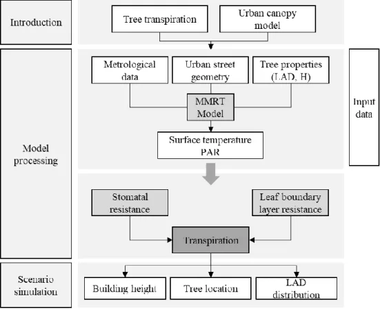
2.1. Research flow
This study focuses on developing a multi-layer model to calculate urban tree transpiration considering vertical structure of trees and building. In scenario simulation, the transpiration is simulated and compared by scenarios varying building height, tree location and leaf area density(LAD) distribution of tree. Fig. 1 presents a flow chart of our methodology.
5
2.2. Model description
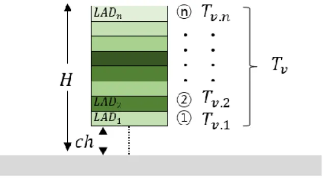
Figure 2 Model base domain
In this study, the multi-layer model reflecting the vertical structure of tree consists of n layers of crown area at intervals of 1m except for the ground level of single tree (Fig. 2). Among the variables needed to calculate the transpiration, 수목의 구조(LAD, height, crown area), leaf surface temperature through MMRT model, and canopy height are given at each layer.
2.2.1. Input data
The main input data for calculating the transpiration are meteorological data and tree properties (Table 1). Meteorological data can be obtained through the surrounding automatic weather station(AWS).
6
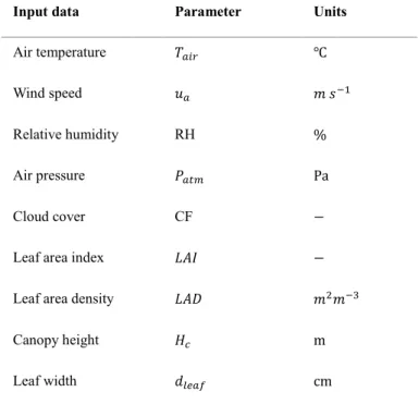
Table 1 Meteorological data, tree properties for input data
Input data Parameter Units
Air temperature 𝑇𝑎𝑖𝑟 ℃
Wind speed 𝑢𝑎 𝑚 𝑠−1
Relative humidity RH %
Air pressure 𝑃𝑎𝑡𝑚 Pa
Cloud cover CF −
Leaf area index 𝐿𝐴𝐼 −
Leaf area density 𝐿𝐴𝐷 𝑚2𝑚−3
Canopy height 𝐻𝑐 m
Leaf width 𝑑𝑙𝑒𝑎𝑓 cm
2.2.2. Model processing
The proposed model to calculate transpiration is based on Ohm's Law resistance analog equation, which is used in many leaf energy flux studies [31,37].
𝑇𝑣=
𝑝𝑎(𝑞𝑠𝑎𝑡(𝑇𝑠)−𝑞𝑎) 𝑟𝑎+𝑟𝑏+𝑟𝑠 (1)
where 𝑞𝑎 (−) is the specific humidity of the air at the reference
height 𝑧𝑎𝑡𝑚 (𝑚), 𝑞𝑠𝑎𝑡(𝑇𝑠) (−) is the specific humidity at saturation at
leaf surface temperature 𝑇𝑠 (℃), 𝑝𝑎 (𝑘𝑔𝑚−3) is air density which can
7
temperature 𝑇𝑎 (℃), and atmospheric pressure 𝑃𝑎𝑡𝑚 (𝑃𝑎), and 𝑟𝑎, 𝑟𝑏
and 𝑟𝑠 ( 𝑠𝑚−1) are the aerodynamic resistance, leaf boundary
resistance and stomatal resistance, respectively.
The specific humidity at saturation and the specific humidity of the air are calculated by Eq. (2) [38]. The air vapor pressure 𝑒𝑎 is calculated with the saturation vapor pressure 𝑒𝑠𝑎𝑡 and relative
humidity RH (%) using Eq. (3). The saturation vapor pressure is calculated using Eq. (4) from Arden-Buck equation [39-40].
𝑞𝑎= 0.622𝑒𝑎/(𝑃𝑎𝑡𝑚− 0.378𝑒𝑎) (2) 𝑒𝑎= 𝑒𝑠𝑎𝑡𝑅𝐻/100 (3) 𝑒𝑠𝑎𝑡 = 100 × 6.1121𝑒𝑥𝑝 (18.678 − T 234.5) ( T 257.14+T) (4)
The transpiration model consists largely of calculating 1) PAR (Photosynthetically Active Radiation, μmol m−2s−1) &, Leaf surface
temperature, 2) Leaf boundary layer resistance 3) Stomatal resistance.
2.2.2.1. PAR & Leaf surface temperature
One of the key part of the model is the calculation of the transpiration using PAR and leaf surface temperature each layer, which is calculated by MMRT model [34]. MMRT model simulates shortwave and longwave radiation exchanges for the view factor between each urban element, with air temperature, dew point, wind
8
speed, cloud cover, and relative humidity. I calculate the shortwave radiation and leaf surface temperature of each layer as MMRT model to reflect the variation in the transpiration caused by different PAR and surface temperatures depending on the location within the tree. The detailed algorithm is described in [34]. As result of MMRT model is shortwave radiation SW (Wm−2) , I multiply 4.57 to convert
unit(μmol m−2s−1, [41]) and 0.45 again because the proportion of
PAR (is often defined as the 400 to 700 nm) in total solar radiation is approximately 45% [42] and many study used it [43-45].
PAR = 4.57 × 0.45 × 𝑆𝑊 (5)
2.2.2.2. Leaf boundary layer resistance
The leaf boundary layer resistance is calculated by the mean plant leaf boundary conductance 𝑔𝑏 (𝑚𝑠−1) using Eq. (6), which is
function of wind speed and therefore of height within the canopy. I follow Eq. (7) from [46] and used by [38,47,48].
𝑟𝑏 = 1/𝑔𝑏 (6)
𝑔𝑏= 𝑎(𝑢(𝐻𝑘)/𝑑𝑙𝑒𝑎𝑓) 1/2
(7)
where 𝑎 = 0.01 (𝑚s−1/2) is an empirical coefficient [47],
𝑑𝑙𝑒𝑎𝑓 (𝑚) is the characteristic leaf dimension, often referred to as
9
The wind speed profile is assumed to be logarithmic above the urban canopy, exponential with in the urban canyon using Eqs. 8-9 [49-51]. 𝑢𝐻𝑐 = 𝑢𝑎 ln (𝐻𝑐𝑧− 𝑑0 𝑜 ) ln (𝑧𝑎𝑡𝑚𝑧− 𝑑0 𝑜 ) (8) 𝑢𝐻𝑘 = 𝑢𝐻𝑐exp (−𝛽 (1 − 𝐻𝑘 𝐻𝑐 )) (9)
where 𝑢𝑎 (𝑚s−1) is the wind speed at reference height and
𝑧𝑜 (𝑚) is the aerodynamic roughness length, which is calculated by
Eq. (9) [49-50].
𝑧𝑜 = 0.1𝐻𝑐 (9)
where 𝑢𝑎 (𝑚s−1) is the wind speed at reference height and 𝛽 (−) is the light extinction parameter, which are calculated from [52]. 𝑑0 (𝑚) and 𝑧𝑜 (𝑚) are the zero displacement height and
aerodynamic roughness length, respectively, which are calculated according to the approach developed by [53] and modified by [54] as follows using Eqs. 10-11:
𝑑0= (1 − αA−𝜆 𝑝 (𝜆𝑝− 1)) 𝐻 𝑐 (10) 𝑧𝑜 = 𝐻𝑐(1 − 𝑑0 𝐻𝑐) exp [− ( 1 𝑘20.5𝛽𝐴𝐶𝐷𝑏(1 − 𝑑0 𝐻𝑐) {𝐴𝑓,𝑏+𝑃𝑣𝐴𝑓,𝑣} 𝐴𝑡𝑜𝑡 ) −0.5 ] (11)
10
where 𝑘 = 0.4 (−) is the von Karman constant, and αA= 0.43 (−),
𝛽𝐴= 1 (−), 𝐶𝐷𝑏= 1.2 (−) are parameter values for staggered arrays
[53]. 𝐻𝑐 (𝑚) is the canopy height, 𝜆𝑝 (−) the plan area index of the
urban roughness elements, 𝐴𝑓,𝑏 (m) the actual frontal area of buildings, 𝐴𝑓,𝑣 (m) the actual frontal area of vegetation, 𝐴𝑡𝑜𝑡 (𝑚) the
total urban plan area, and 𝑃𝑣 (– ) the ratio between vegetation drag
𝐶𝐷𝑣 and building drag 𝐶𝐷𝑏. These parameters are calculated from [51,
54-56]. For volumetric/aerodynamic porosity, light extinction parameter is calculated as [57], assuming spherical leaf angle distribution.
2.2.2.3. Aerodynamic resistance
The aerodynamic resistance is calculated by simpler method [38], which assume neutral condition as follows using Eqs. 12-13:
𝑟𝑎= 1 𝑘2𝑢 𝐻𝑘[ ln(𝑧𝑎𝑡𝑚−𝑑0) 𝑧𝑜 ] [ ln(𝑧𝑎𝑡𝑚−𝑑0) 𝑧𝑜ℎ ] (12) 𝑧𝑜ℎ = 0.1𝑧𝑜 (13)
where 𝑧𝑜ℎ (𝑚) is the roughness length for heat.
2.2.2.4. Stomatal resistance
As reciprocal of stomatal conductance is stomatal resistance, stomatal conductance 𝑔𝑠 (mol m−2s−1) is caculated first. Many
11
studies reported that stomatal conductance was closely coupled with leaf photosynthesis [58-59]. In proposed model, stomatal conductance is calculated as a function of leaf photosynthesis 𝐴𝑛 (μmol m−2s−1) by Eq. (14) from [60] used by [31,59,61].
𝑔𝑠=
m𝐴𝑛ℎ𝑠
𝐶𝑠
+ 𝑔0 (14)
where m (−) is the slope, 𝑔0 (mol m−2s−1) is the zero intercept,
ℎ𝑠 and 𝐶𝑠 (𝑝𝑝𝑚) are, respectively, relative humidity and CO2
concentration at the leaf surface. In this model, modified equation is used from [62], by using CO2 concentration 𝐶𝑎 (𝑝𝑝𝑚) , relative humidity rh (-) in the air as follows using Eq. (15):
𝑔𝑠=
m𝐴𝑛𝑟ℎ
𝐶𝑎
+ 𝑔0 (15)
The leaf photosynthesis is simulated according to [63]. The version of the model proposed by [62] was used, which is calculating photosynthesis without including the potential limitation arising from triose phosphate utilization, and is used by [37,64].
𝐴𝑛= [1 −
0.5𝑂
𝜏𝐶𝑖 ] min(𝑊𝑐
, 𝑊𝑗) − 𝑅𝑑 (16)
where 𝑊𝑐 (μmol m−2s−1) is the carboxylation rate when ribulose bisphosphate(RuBP) is saturated, 𝑊𝑗 (μmol m−2s−1) is the
12
carboxylation rate when RuBP regeneration is limited by electron transport, 𝜏 is the specificity factor for Rubisco [65], 𝑅𝑑 (μmol m−2s−1) is the rate of 𝐶𝑂2 evolution in light that results
from processes other than photorespiration, and 𝑂 and 𝐶𝑖 (Pa) are
the partial pressures of 𝑂2 and 𝐶𝑂2 in interior leaf, respectively. In proposed model, 𝐶𝑖/𝐶𝑎= 0.7 is used, where 𝐶𝑎 (𝑃𝑎) is partial
pressures of 𝐶𝑂2 in air, which is what is typically observed in C3 plants under favorable conditions [58,66,67].
𝑊𝑐 obeys competitive Michaelis-Menten kinetics with respect to
𝐶𝑂2 and 𝑂2 as follows using Eq. (17):
𝑊𝑐=
𝑉𝑐𝑚𝑎𝑥𝐶𝑖
𝐶𝑖+ 𝐾𝑐(1 +𝐾O 𝑜)
(17)
where 𝑉𝑐𝑚𝑎𝑥 (μmol m−2s−1) is the maximum rate of
carboxylation, and 𝐾𝑐 and 𝐾𝑜 (Pa) are Michaelis constants of
Rubisco for carboxylation and oxygenation, respectively.
𝑊𝑗 is controlled by the rate of electron transport J (μmol m−2s−1)
which depends on PAR, which are calculated as follows using Eqs. 18-19: 𝑊𝑗= J𝐶𝑖 4 (𝐶𝑖+O𝜏 ) (18) J = α × PAR (1 +α2PAR2 𝐽𝑚𝑎𝑥2 ) 1/2 (19)
13
where 𝐽𝑚𝑎𝑥 (μmol m−2s−1) is the light-saturated rate of electron transport, and α is the quantum yield that means efficiency of light energy conversion on an incident light basis.
The coefficients for 𝑉𝑐𝑚𝑎𝑥, 𝐽𝑚𝑎𝑥, 𝐾𝑐, 𝐾𝑜, 𝑅𝑑 and 𝜏 are strong,
non-linear functions of temperature [68-69]. One temperature function used for 𝐾𝑐, 𝐾𝑜, 𝑅𝑑 and 𝜏 is Eq. (20) from [62]:
Parameter(𝐾𝑐, 𝐾𝑜, 𝑅𝑑, 𝜏) = exp (c − ∆Ha/RTs′) (20)
where c (−) is a dimensionless, scaling constant, ∆Ha (J mol−1) is an activation energy, R (8.3143JK−1mol−1) is the gas constant and
𝑇𝑠′ (𝐾) is a leaf surface temperature. The temperature dependence
of 𝑉𝑐𝑚𝑎𝑥 and 𝐽𝑚𝑎𝑥 is Eq. (21) from [62,70]:
Parameter(𝑉𝑐𝑚𝑎𝑥, 𝐽𝑚𝑎𝑥) =
exp (c − ∆Ha/RTs′)
1 + exp [(∆S𝑇𝑠′− ∆Hd)/(𝑅Ts′)]
(21)
where ∆Hd (J mol−1) is an energy of deactivation and
∆S (JK−1mol−1) is an entropy term. The linear relationships commonly observed between leaf photosynthetic capacities and amount of leaf nitrogen on an area basis Na (g m−2) [62,71-73]. To account for
linear relationships, the scaling factors c for 𝑉𝑐𝑚𝑎𝑥, 𝐽𝑚𝑎𝑥, 𝑅𝑑 is
calculated by Eq. (22) from [64].
14
In proposed model, the amount of leaf nitrogen is estimated from daily PAR intercepted by leaves PARi (mol m−2d−1) by an empirical
linear relationship Eq. (23) from [74].
𝑁𝑎= aNa+ 𝑏𝑁𝑎𝑃𝐴𝑅𝑖 (23)
The stomatal resistance through stomatal conductance of Eq. (10) is expressed in biochemical units of (m2s mol−1). The conversion to
common units (s m−1) for Eq. (1) is obtained as follows using Eq.
(24) from [75]:
𝑟𝑠(𝑠𝑚−1) =
Tf 𝑃𝑎𝑡𝑚
0.0224𝑇𝑠′ 𝑃𝑎𝑡𝑚,0
𝑟𝑠(m2s mol−1) (24)
where Tf= 273.15 (𝐾) is the freezing temperature and 𝑃𝑎𝑡𝑚,0=
101325 (Pa) is a reference atmospheric pressure.
A complete list of the parameters for calculating resistances is given in Table 3.
15
2.3. Scenario simulation
I simulate PAR, leaf surface temperature and finally transpiration to evaluate and compare various scenarios including height of buildings surrounding the tree, location of tree and LAD distribution of each layer. Model parameters of MMRT model are listed in the Appendix.
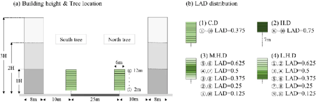
The domain for simulation is presented in Fig. 4. In the domain, two building, two sidewalks, one road, two trees, and the width and height of which are denoted in domain. The tree height is 12m, tree crown width is 6m, and tree vertical layer thickness is 1m.
Figure 3 Domain for simulation
2.3.1. Tree location
Transpiration can be varied by tree position with building because of solar radiance absorption. To evaluate the differences depending on the location of the tree, the E-W street is set making that two trees locate northern and southern (Fig. 4a), respectively.
16 2.3.2. Building height
The building environment surrounding trees affect transpiration [76], for example, reflecting radiation, intercepting shortwave radiation, emitting longwave radiation and changing canopy height. The intensity of the urban heat island changes with height/width ratio [77]. To evaluate the effect of various building environment, we control building height in three cases (1H, 2H, and 3H). Case 1H is an urban canyon with 12m buildings; case 2H is an urban canyon with 24m buildings; and case 3H is an urban canyon with 36m buildings. H means tree canopy height.
2.3.3. LAD distribution
Higher LAI of tree must lead higher transpiration. LAD distribution, however, can be various cases in same LAI. We evaluate the transpiration for four vertical structure cases; (1) Constant Density (C.D), (2) High Density, few layers (H.D), (3) High Density in Middle layers (M.H.D), (4) High Density in lower layers (L.H.D). LAI and tree height is same in all cases. The crown base height of H.D case is 7m, while other cases are 2m to make same LAI (Fig. 4b)
For the simulation, I select the 213th day of the year (DOY, 1 August) in 2018 in Seoul (126.9658, 37.57142). 213 DOY was a clear day and did not have rain back and forth. It also had high air
17
temperature, low relative humidity that led to higher transpiration, so that I can see difference of transpiration rate with different condition. Table 2 shows the input data for the simulations. For the simulation, O (Pa), 𝐶𝑎 (ppm) are set as 21000 and 401.91 [78], respectively.
Vertical variations of RH, 𝐶𝑎 are ignored because variations are relatively small and varies with stable condition of air [79-81].
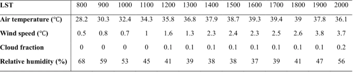
Table 2 Meteorological data for the model simulation
Values of the main parameters and reference used in the simulation are given in Table 3. To compare transpiration of all case relatively, parameters for calculating resistances are fixed and mainly derived by [62,64]. The leaf width 𝑑𝑙𝑒𝑎𝑓 is set as 7.5cm of
Ginkgo biloba which is planted largest proportion of street tree in Seoul [82]. LST 800 900 1000 1100 1200 1300 1400 1500 1600 1700 1800 1900 2000 Air temperature (℃) 28.2 30.3 32.4 34.3 35.8 36.8 37.9 38.7 39.3 39.4 39 37.8 36.1 Wind speed (℃) 0.5 0.8 0.7 1 1.6 1.3 2.3 2.4 2.3 2.5 2.6 3.8 3.7 Cloud fraction 0 0 0 0 0.1 0.1 0.1 0.1 0.1 0.1 0.1 0.1 0.2 Relative humidity (%) 68 59 53 45 41 39 38 38 37 39 41 47 56
18
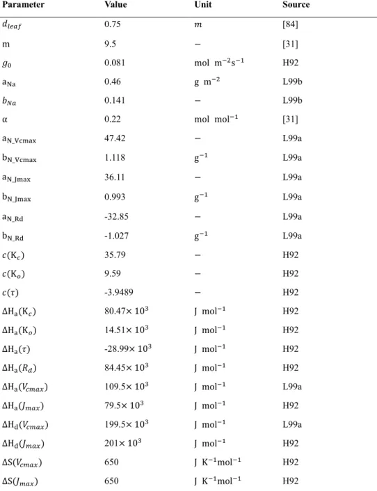
Table 3 Values, units and sources of the parameters for resistances
Parameter Value Unit Source
𝑑𝑙𝑒𝑎𝑓 0.75 𝑚 [84] m 9.5 − [31] 𝑔0 0.081 mol m−2s−1 H92 aNa 0.46 g m−2 L99b 𝑏𝑁𝑎 0.141 − L99b α 0.22 mol mol−1 [31] aN_Vcmax 47.42 − L99a bN_Vcmax 1.118 g−1 L99a aN_Jmax 36.11 − L99a bN_Jmax 0.993 g−1 L99a aN_Rd -32.85 − L99a bN_Rd -1.027 g−1 L99a 𝑐(K𝑐) 35.79 − H92 𝑐(K𝑜) 9.59 − H92 𝑐(𝜏) -3.9489 − H92 ∆Ha(K𝑐) 80.47× 10³ J mol−1 H92 ∆Ha(K𝑜) 14.51× 10³ J mol−1 H92 ∆Ha(𝜏) -28.99× 10³ J mol−1 H92 ∆Ha(𝑅𝑑) 84.45× 10³ J mol−1 H92 ∆Ha(𝑉𝑐𝑚𝑎𝑥) 109.5× 10³ J mol−1 L99a ∆Ha(𝐽𝑚𝑎𝑥) 79.5× 10³ J mol−1 H92 ∆Hd(𝑉𝑐𝑚𝑎𝑥) 199.5× 10³ J mol−1 L99a ∆Hd(𝐽𝑚𝑎𝑥) 201× 103 J mol−1 H92 ∆S(𝑉𝑐𝑚𝑎𝑥) 650 J K−1mol−1 H92 ∆S(𝐽𝑚𝑎𝑥) 650 J K−1mol−1 H92 Sources: H92=[62], L99a=[64], L99b=[74].
19
Chapter 3. Results and Discussion
3.1. Parameter
3.1.1. PAR & leaf surface temperature
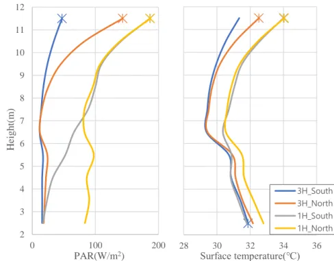
Figure 4 Vertical profile of PAR(left) and leaf surface temperature(right) according to tree location(south, north) / building height(1H,3H). (LAD
distribution: C.D, time: 15h and *: maximum value, 38.7 2.4 0.1 37)
The results of PAR and leaf surface temperature simulated by MMRT model are shown in Fig. 4. When the building is low(1H), higher PAR and surface temperature are resulted. PAR shows decreasing shape depending on the height, but the vertical profile of surface temperature is not. The highest surface temperature usually is in the upper layer, but the lower layer close to the ground is upper
2 3 4 5 6 7 8 9 10 11 12 0 100 200 Heig h t( m ) PAR(W/m2) 28 30 32 34 36 Surface temperature(℃) 3H_South 3H_North 1H_South 1H_North
20
than the middle layer due to high longwave radiation emitted from ground. This is similar to higher results as the surface temperature of the tree trunk nears the surface [77]. The pattern is obvious in the 3H, South tree, where solar radiation is largely intercepted by the building, resulting in small difference between high layer and low layer. This pattern makes a different vertical profile of surface temperature, which is slightly higher at first layer than top layer.
3.1.2. Resistances
Figure 5 Vertical profile of leaf boundary layer resistance(left) and stomatal resistance(right) according to building height(1H, 2H, 3H, north tree), tree location(south, north, 1H), respectively. (LAD distribution: C.D, time: 15h)
Data in Fig. 5 show vertical profiles of leaf boundary layer resistance
2 3 4 5 6 7 8 9 10 11 12 0 50 100 Heig h t( m )
Boundary layer resistance (s/m)
1H 2H 3H 0 200 400 600 Stomatal resistance(s/m) South North
21
and stomatal resistance. In the upper layer, it is showed relatively high wind speed and PAR, resulting in lower both resistance. In scenario of 3H, as the height decreases, the wind speed decreases significantly due to high canopy height, resulting in a large difference in boundary layer resistance.
3.2. Transpiration
3.2.1. Temporal variation
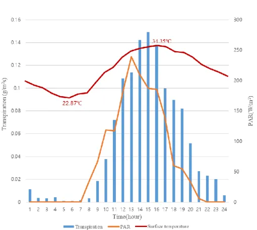
Figure 6 Temporal variation of tree transpiration rate(bar) with PAR(orange line) and surface temperature(red line) of top layer (building height: 1H, tree
location: north, LAD distribution: C.D)
22
with PAR and leaf surface temperature. Despite the highest PAR causing the lowest stomatal resistance, it does not show the highest result transpiration rate at the time with highest PAR. This is because the temporal pattern of leaf surface temperature, another factor that has a dominant effect on transpiration, does not perfectly match PAR pattern. Therefore, transpiration rate is high at the time that the surface temperature and PAR are simultaneously high.
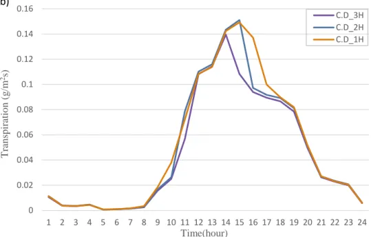
3.2.2. Scenarios simulation 0 0.02 0.04 0.06 0.08 0.1 0.12 0.14 0.16 1 2 3 4 5 6 7 8 9 10 11 12 13 14 15 16 17 18 19 20 21 22 23 24 T ran sp ir atio n ( g /m 2s) Time(hour) C.D_3H C.D_2H C.D_1H (a)
23
Figure 7 Transpiration rate changes by the building height scenarios during a day (1H, 2H, 3H). (a) South tree (b) North tree. (LAD distribution: C.D)
In all of the tree location scenarios, the lower height of the surrounding buildings, the higher the transpiration rate (Fig. 7). The difference of transpiration rate mainly occurs at the time daytime. However, the variation of south tree is higher than north tree according to building height. In the C.D LAD distribution scenarios, the difference in tree transpiration during a day is up to 24.1%(south), 13.2%(north) depending on the building height (Fig. 7). The south tree is more sensitive to the height of the building because it is close to the building that forms the shadow.
0 0.02 0.04 0.06 0.08 0.1 0.12 0.14 0.16 1 2 3 4 5 6 7 8 9 10 11 12 13 14 15 16 17 18 19 20 21 22 23 24 T ran sp ir atio n ( g /m 2s) Time(hour) C.D_3H C.D_2H C.D_1H (b)
24
Figure 8 Transpiration rate changes by LAD distribution, tree location, building height scenarios
Fig. 8 shows the total transpiration rate during the day according to all scenarios for four LAD distributions, two tree locations and three building heights. Depending on the scenarios, the LAD distribution of the most evaporating trees differed, which means that the most efficient/inefficient trees vary depending on urban space and the arrangement of trees. In particular, it is noteworthy that the H.D. case, which has high LAD density, results in most efficiency at 3H scenarios and worst efficiency at 1H scenarios, regardless of tree location.
Fig. 8 shows that the LAD distribution of trees is relatively important in environment with high building. In scenario where building height are high(3H), the variations in tree transpiration
3 3.2 3.4 3.6 3.8 4 4.2 4.4 4.6
1H_South 1H_North 2H_South 2H_North 3H_South 3H_North
T ran sp ir atio n r ate (k g /m 2/d ay ) C.D H.D M.H.D L.H.D Mean
25
during a day is up to 8.3%(south) and 5.6%(north) according to LAD distribution. In scenario of 1H, the variations are 7.4%(south) and 6.5%(north). In addition, the difference between north and south trees is greater if the building is high compared low (14.4% in 3H, 6.2% in 1H).
The results of scenario simulation suggest that the location and shape of trees that are efficient for cooling, vary depending on the urban environment. This model can better evaluate the cooling effect of trees by considering the radiant heat intercepting effect of trees. For example, the shallow canyon can be hotter due to high exposure of the canyon's surfaces to the intense solar radiation [77,84]. And the air temperature with taller buildings are lower due to their shading effect [85]. Therefore, in consideration of that the shallow street canyon need higher cooling effect, the tree which have big crown could be effective in terms of both of transpiration and shading [86-87]. The results can be used to design street tree for improved thermal comfort when used with air temperature, humidity, and wind speed.
3.3. Model limitations and future development
This study proposes a multi-layer model that considers the vertical structure of trees and building to calculate the transpiration rate of urban trees. That generates difference between the vapor pressure deficit, wind speed, and resistance values, which makes in
26
turn difference result of transpiration depending on the scenarios. Although many parameters which can lead to restrictive result are fixed to simulate transpiration, it is meaningful to compare the relative transpiration rate of each scenarios. Future studies need to estimate and verify parameters of model to improve accuracy.
And the MMRT model would calculate the surface temperature higher than it actually is because it has limitations in processing latent heat, making the latent heat very small by using a very large Bowen ratio. Thus, in order to increase accuracy, this limit could be developed through feedback that calculates latent heat using transpiration of proposed model and calculates surface temperature again.
This study only dealt with the transpiration of tree cooling effects. Considering the radiative heat reduction of tree in the future, it will be a more accurate assessment of the cooling effect of trees. Under various conditions, there will be different cooling requirements, along with other thermal environments, and the shadow effects will vary significantly.
The model used only one day of weather conditions which can lead to only one case. If I simulate on days with low temperatures and high humidity, the difference may be small in each case.
27
Chapter 4. Conclusion
I propose a multi-layer model for calculating transpiration of urban trees. The advantage of the model is that it simulates transpiration considering the vertical structure of trees and building. To reflect vertical structure effectively, PAR and leaf surface temperature data simulated by MMRT model, one of the urban canopy model. The proposed model includes a detailed representation of plant biophysical and echophysiological characteristics.
Simulations are conducted on four LAD distribution of trees with three types of building (12m, 24m, and 36m) and two types of tree location (South and North). North tree surrounded by low building is most efficient for transpiration. The difference in tree transpiration during a day is up to 24.1%(south), 13.2%(north) depending on the building height. In scenario where building height are high(3H) and low(1H), the variations in tree transpiration during a day is up to 8.3% (3H) and 7.4%(1H) according to LAD distribution. It is similar respect to tree location.
The scenario simulation suggests that the location and shape of trees that are efficient for cooling effect, vary depending on the urban environment. This model is useful tool providing guideline on the plantation of thermo-efficient trees depending on the structure or environment of the city If I analyze transpiration and radiant heat reduction effects together in future studies, it will be able to gain more accurate insight into the cooling effects of trees.
28
Bibliography
[1] J. O’Loughlin, F.D.W. Witmer, A.M. Linke, A. Laing, A. Gettelman, J. Dudhia, Climate variability and conflict risk in East Africa, 1990-2009, Proc. Natl. Acad. Sci. U. S. A. 109 (2012) 18344–18349.
https://doi.org/10.1073/pnas.1205130109.
[2] P. Hoffmann, O. Krueger, K.H. Schlünzen, A statistical model for the urban heat island and its application to a climate change scenario, Int. J. Climatol. 32 (2012) 1238–1248. https://doi.org/10.1002/joc.2348.
[3] D.E. Parker, Urban heat island effects on estimates of
observed climate change, Wiley Interdiscip. Rev. Clim. Chang. 1 (2010) 123–133. https://doi.org/10.1002/wcc.21.
[4] H. Radhi, F. Fikry, S. Sharples, Impacts of urbanisation on the thermal behaviour of new built up environments: A scoping study of the urban heat island in Bahrain, Landsc. Urban Plan. 113 (2013) 47–61.
https://doi.org/10.1016/j.landurbplan.2013.01.013.
[5] D. Armson, P. Stringer, A.R. Ennos, The effect of tree shade and grass on surface and globe temperatures in an urban area, Urban For. Urban Green. 11 (2012) 245–255. https://doi.org/10.1016/j.ufug.2012.05.002.
[6] A.H. Block, S.J. Livesley, N.S.G. Williams, Responding to the Urban Heat Island : A Review of the Potential of Green Infrastructure, Vic. Cent. Clim. Chang. Adapt. (2012) 1–62. http://staging.202020vision.com.au/media/1026/responding- to-the-urban-heat-island-a-review-of-the-potential-of-green-infrastructure.pdf.
29
[7] K.R. Gunawardena, M.J. Wells, T. Kershaw, Utilising green and bluespace to mitigate urban heat island intensity, Sci. Total Environ. 584–585 (2017) 1040–1055.
https://doi.org/10.1016/j.scitotenv.2017.01.158.
[8] J. Konarska, F. Lindberg, A. Larsson, S. Thorsson, B. Holmer, Transmissivity of solar radiation through crowns of single urban trees-application for outdoor thermal comfort modelling, Theor. Appl. Climatol. 117 (2014) 363–376. https://doi.org/10.1007/s00704-013-1000-3.
[9] J. Konarska, J. Uddling, B. Holmer, M. Lutz, F. Lindberg, H. Pleijel, S. Thorsson, Transpiration of urban trees and its cooling effect in a high latitude city, Int. J. Biometeorol. 60 (2016) 159–172. https://doi.org/10.1007/s00484-015-1014-x.
[10] Z. Tan, K.K.L. Lau, E. Ng, Urban tree design approaches for mitigating daytime urban heat island effects in a high-density urban environment, Energy Build. 114 (2016) 265–274. https://doi.org/10.1016/j.enbuild.2015.06.031.
[11] Y. Wang, H. Akbari, The effects of street tree planting on Urban Heat Island mitigation in Montreal, Sustain. Cities Soc. 27 (2016) 122–128.
https://doi.org/10.1016/j.scs.2016.04.013.
[12] P.A. Mirzaei, F. Haghighat, Approaches to study Urban Heat Island - Abilities and limitations, Build. Environ. 45 (2010) 2192–2201. https://doi.org/10.1016/j.buildenv.2010.04.001. [13] M.A. Rahman, A. Moser, A. Gold, T. Rötzer, S. Pauleit,
Vertical air temperature gradients under the shade of two contrasting urban tree species during different types of summer days, Sci. Total Environ. 633 (2018) 100–111.
30
https://doi.org/10.1016/j.scitotenv.2018.03.168.
[14] H. Akbari, Shade trees reduce building energy use and CO2 emissions from power plants, Environ. Pollut. 116 (2002) 119–126. https://doi.org/10.1016/S0269-7491(01)00264-0. [15] B.S. Lin, Y.J. Lin, Cooling effect of shade trees with
different characteristics in a subtropical urban park, HortScience. 45 (2010) 83–86.
https://doi.org/10.21273/hortsci.45.1.83.
[16] H. Taha, Urban climates and heat islands: Albedo,
evapotranspiration, and anthropogenic heat, Energy Build. 25 (1997) 99–103.
https://doi.org/10.1016/s0378-7788(96)00999-1.
[17] C. Campillo, R. Fortes, M. del Henar Prieto, Solar Radiation Effect on Crop Production, Sol. Radiat. (2012).
https://doi.org/10.5772/34796.
[18] M. Ballinas, V.L. Barradas, The Urban Tree as a Tool to Mitigate the Urban Heat Island in Mexico City: A Simple Phenomenological Model, J. Environ. Qual. 45 (2016) 157– 166. https://doi.org/10.2134/jeq2015.01.0056.
[19] Y. Wang, H. Akbari, The effects of street tree planting on Urban Heat Island mitigation in Montreal, Sustain. Cities Soc. 27 (2016) 122–128.
https://doi.org/10.1016/j.scs.2016.04.013.
[20] G. Kim, P. Coseo, Urban park systems to support
sustainability: The role of urban park systems in hot arid urban climates, Forests. 9 (2018) 1–16.
https://doi.org/10.3390/f9070439.
[21] Y. Dai, R.E. Dickinson, Y.P. Wang, A two-big-leaf model for canopy temperature, photosynthesis, and stomatal
31
conductance, J. Clim. 17 (2004) 2281–2299.
https://doi.org/10.1175/1520-0442(2004)017<2281:ATMFCT>2.0.CO;2.
[22] J.L. Monteith, Solar Radiation and Productivity in Tropical Ecosystems, J. Appl. Ecol. 9 (1972) 747.
https://doi.org/10.2307/2401901.
[23] T.A. McMahon, M.C. Peel, L. Lowe, R. Srikanthan, T.R. McVicar, Estimating actual, potential, reference crop and pan evaporation using standard meteorological data: A pragmatic synthesis, Hydrol. Earth Syst. Sci. 17 (2013) 1331–1363. https://doi.org/10.5194/hess-17-1331-2013.
[24] P.S. Nobel, Photosynthetic Rates of Sun versus Shade Leaves of Hyptis emoryi Torr. , Plant Physiol. 58 (1976) 218–223. https://doi.org/10.1104/pp.58.2.218.
[25] T.L. Pons, W. Jordi, D. Kuiper, Acclimation of plants to light gradients in leaf canopies: Evidence for a possible role for cytokinins transported in the transpiration stream, J. Exp. Bot. 52 (2001) 1563–1574.
https://doi.org/10.1093/jexbot/52.360.1563.
[26] M. Saudreau, A. Ezanic, B. Adam, R. Caillon, P. Walser, S. Pincebourde, Temperature heterogeneity over leaf surfaces: the contribution of the lamina microtopography, Plant Cell Environ. 40 (2017) 2174–2188.
https://doi.org/10.1111/pce.13026.
[27] T.R. Sinclair, C.E. Murphy, K.R. Knoerr, Development and Evaluation of Simplified Models for Simulating Canopy Photosynthesis and Transpiration, Br. Ecol. Soc. 13 (1976) 813–829. https://www.jstor.org/stable/2402257.
32
conductance, photosynthesis and partitioning of available energy I: Model description and comparison with a multi-layered model, Agric. For. Meteorol. 91 (1998) 89–111. https://doi.org/10.1016/S0168-1923(98)00061-6. [29] [1] R. LEUNING, A critical appraisal of a combined
stomatal‐photosynthesis model for C3 plants, Plant. Cell Environ. 18 (1995) 339–355. https://doi.org/10.1111/j.1365-3040.1995.tb00370.x.
[30] R.D. Pyles, B.C. Weare, K.T. Pawu, The UCD advanced canopy- atmosphere-soil algorithm: Comparisons with observations from different climate and vegetation regimes, Q. J. R. Meteorol. Soc. 126 (2000) 2951–2980.
https://doi.org/10.1256/smsqj.56916.
[31] D.D. Baldocchi, K.B. Wilson, L. Gu, How the environment, canopy structure and canopy physiological functioning influence carbon, water and energy fluxes of a temperate broad-leaved deciduous forest - An assessment with the biophysical model CANOAK, Tree Physiol. 22 (2002) 1065– 1077. https://doi.org/10.1093/treephys/22.15-16.1065. [32] Z.H. Wang, E. Bou-Zeid, J.A. Smith, A coupled energy
transport and hydrological model for urban canopies evaluated using a wireless sensor network, Q. J. R. Meteorol. Soc. 139 (2013) 1643–1657. https://doi.org/10.1002/qj.2032.
[33] Y.H. Ryu, E. Bou-Zeid, Z.H. Wang, J.A. Smith, Realistic Representation of Trees in an Urban Canopy Model, Boundary-Layer Meteorol. 159 (2016) 193–220. https://doi.org/10.1007/s10546-015-0120-y.
[34] C.Y. Park, D.K. Lee, E.S. Krayenhoff, H.K. Heo, S. Ahn, T. Asawa, A. Murakami, H.G. Kim, A multilayer mean radiant
33
temperature model for pedestrians in a street canyon with trees, Build. Environ. 141 (2018) 298–309.
https://doi.org/10.1016/j.buildenv.2018.05.058.
[35] H.C. Ward, S. Kotthaus, L. Järvi, C.S.B. Grimmond, Surface Urban Energy and Water Balance Scheme (SUEWS):
Development and evaluation at two UK sites, Urban Clim. 18 (2016) 1–32. https://doi.org/10.1016/j.uclim.2016.05.001. [36] K.A. Nice, A.M. Coutts, N.J. Tapper, Development of the
VTUF-3D v1.0 urban micro-climate model to support assessment of urban vegetation influences on human thermal comfort, Urban Clim. 24 (2018) 1052–1076.
https://doi.org/10.1016/j.uclim.2017.12.008.
[37] H. Sinoquet, X. Le Roux, B. Adam, T. Ameglio, F.A. Daudet, RATP: A model for simulating the spatial distribution of radiation absorption, transpiration and photosynthesis within canopies: Application to an isolated tree crown, Plant, Cell Environ. 24 (2001) 395–406. https://doi.org/10.1046/j.1365-3040.2001.00694.x.
[38] S. Fatichi, The modeling of hydrological cycle and its interaction with vegetation in the framework of climate change, Univ. Firenze. (2010) 463.
[39] A.L. Buck, New equations for computing vapour pressure and enhancement factor., J. Appl. Meteorol. 20 (1981) 1527– 1532.
https://doi.org/10.1175/1520-0450(1981)0202.0.CO;2.
[40] Buck Research Instruments, Humidity conversion equations, Model CR-1A Hygrom. with Autofill, Oper. Man. (2012) 20– 21. http://www.hygrometers.com/wp-content/uploads/CR-1A-users-manual-2009-12.pdf.
34
[41] J.C. Sager, J.C.M. Farlane, Chapter 1. Radiation, Growth Chamb. Handb. 46 (2003) 30–33.
https://doi.org/http://doi.acm.org/10.1145/636772.636794. [42] W. Larcher, 1995. Physiological plant ecology, 3rd Edn.
Springer- Verlag, Heidelberg, 506 p
[43] T.L. Ginter, Shade Adaptive Responses of Plants, Texas Tech U Diversity, 2001.
[44] S. Smolander, P. Stenberg, A method for estimating light interception by a conifer shoot, Tree Physiol. 21 (2001) 797– 803. https://doi.org/10.1093/treephys/21.12-13.797.
[45] M. He, J.S. Kimball, M.P. Maneta, B.D. Maxwell, A. Moreno, S. Beguería, X. Wu, Regional crop gross primary productivity and yield estimation using fused landsat-MODIS data, Remote Sens. 10 (2018). https://doi.org/10.3390/rs10030372.
[46] H.G. Jones, Plants and Microclimate, Cambridge University Press, New York.
[47] B.J. Choudhury, J.L. Monteith, A four‐layer model for the heat budget of homogeneous land surfaces, Q. J. R. Meteorol. Soc. 114 (1988) 373–398.
https://doi.org/10.1002/qj.49711448006.
[48] W.J. Shuttleworth, R.J. Gurney, The theoretical relationship between foliage temperature and canopy resistance in sparse crops, Q. J. R. Meteorol. Soc. 116 (1990) 497–519.
https://doi.org/10.1002/qj.49711649213.
[49] V. Masson, A physically-based scheme for the urban energy budget in atmospheric models, Boundary-Layer Meteorol. 94 (2000) 357–397.
https://doi.org/10.1023/A:1002463829265.
35
below-canopy representations of turbulent fluxes in an energy balance snowmelt model, Water Resour. Res. 49 (2013) 1107–1122. https://doi.org/10.1002/wrcr.20073. [51] N. Meili, G. Manoli, P. Burlando, E. Bou-Zeid, W.T.L. Chow,
A.M. Coutts, E. Daly, K.A. Nice, M. Roth, N.J. Tapper, E. Velasco, E.R. Vivoni, S. Fatichi, An urban ecohydrological model to quantify the effect of vegetation on urban climate and hydrology (UT&C v1.0), Geosci. Model Dev. 13 (2020) 335–362. https://doi.org/10.5194/gmd-13-335-2020.
[52] J.L. Wright, Evaluating turbulent transfer aerodynamically within the microclimate of a cornfield, Univ. Cornell. (1965) 174.
[53] R.W. Macdonald, R.F. Griffiths, D.J. Hall, An improved method for the estimation of surface roughness of obstacle arrays, Atmos. Environ. 32 (1998) 1857–1864.
https://doi.org/10.1016/S1352-2310(97)00403-2.
[54] C.W. Kent, S. Grimmond, D. Gatey, Aerodynamic roughness parameters in cities: Inclusion of vegetation, J. Wind Eng. Ind. Aerodyn. 169 (2017) 168–176.
https://doi.org/10.1016/j.jweia.2017.07.016.
[55] G. De-xin, Z. Ting-yao, H. Shi-jie, Wind tunnel experiment of drag of isolated tree models in surface boundary layer, J. For. Res. 11 (2000) 156–160.
https://doi.org/10.1007/BF02855516.
[56] D. Guan, Y. Zhang, T. Zhu, A wind-tunnel study of windbreak drag, Agric. For. Meteorol. 118 (2003) 75–84. https://doi.org/10.1016/S0168-1923(03)00069-8.
36
for Canopy Temperature, Photosynthesis, and Stomatal Conductance, J. Clim. 17 (2004) 2281–2299.
https://doi.org/10.1175/1520-0442(2004)017<2281:ATMFCT>2.0.CO;2.
[58] S.C. Wong, I.R. Cowan, G.D. Farquhar, Stomatal conductance correlates with photosynthetic capacity, Nature. 282 (1979) 424–426. https://doi.org/10.1038/282424a0.
[59] G.J. Collatz, J.T. Ball, C. Grivet, J.A. Berry, Physiological and environmental regulation of stomatal conductance,
photosynthesis and transpiration: a model that includes a laminar boundary layer, Agric. For. Meteorol. 54 (1991) 107– 136. https://doi.org/10.1016/0168-1923(91)90002-8. [60] J.T. Ball, J.A. Berry, An analysis and concise description of
stomatal responses to multiple environmental factors. Planta, in press.
[61] D. Baldocchi, T. Meyers, On using eco-physiological, micrometeorological and biogeochemical theory to evaluate carbon dioxide, water vapor and trace gas fluxes over
vegetation: A perspective, Agric. For. Meteorol. 90 (1998) 1– 25. https://doi.org/10.1016/S0168-1923(97)00072-5. [62] P.C. HARLEY, R.B. THOMAS, J.F. REYNOLDS, B.R. STRAIN,
Modelling photosynthesis of cotton grown in elevated CO2, Plant. Cell Environ. 15 (1992) 271–282.
https://doi.org/10.1111/j.1365-3040.1992.tb00974.x. [63] G.D. Farquhar, S. von Caemmerer, J.A. Berry, A biochemical
model of photosynthetic CO2 assimilation in leaves of C3 species, Planta. 149 (1980) 78–90.
https://doi.org/10.1007/BF00386231.
37
Parameterization and testing of a biochemically based photosynthesis model for walnut (Juglans regia) trees and seedlings, Tree Physiol. 19 (1999) 481–492.
https://doi.org/10.1093/treephys/19.8.481.
[65] D.B. Jordan, W.L. Ogren, The CO 2 /O 2 specificity of ribulose 1,5-bisphosphate carboxylase/oxygenase - Dependence on ribulosebisphosphate concentration, pH and temperature, Planta. 161 (1984) 308–313.
https://doi.org/10.1007/BF00398720.
[66] A.M. Hetherington, F. l. Woodward, The role of stomata in sensing and driving environmental change, Nature. 424 (2003) 528–539.
https://doi.org/10.4135/9781446201091.n40.
[67] I.C. Prentice, N. Dong, S.M. Gleason, V. Maire, I.J. Wright, Balancing the costs of carbon gain and water transport: Testing a new theoretical framework for plant functional ecology, Ecol. Lett. 17 (2014) 82–91.
https://doi.org/10.1111/ele.12211.
[68] I.R. JOHNSON, J.H.M. THORNLEY, Temperature Dependence of Plant and Crop Process, Ann. Bot. 55 (1985) 1–24.
https://doi.org/10.1093/oxfordjournals.aob.a086868. [69] P.C. Harley, J.D. Tenhunen, Modeling the photosynthetic
response of C3 leaves to environmental factors. Modeling Photosynthesis—From Biochemistry to Canopy. Am. Soc. Agronomy. Madison (1991) 17–39.
https://doi.org/10.2135/cssaspecpub19.c2
[70] F. Johnson, H. Eyring, R. Williams, The nature of enzyme inhibitions in bacterial luminescence: Sulfanilamide, urethane, temperature and pressure, Jotirnal Cell Cotnparative Physiol.
38 20 (1942) 247–268.
https://doi.org/https://doi.org/10.1002/jcp.1030200302. [71] C. Field, Allocating leaf nitrogen for the maximization of
carbon gain: Leaf age as a control on the allocation program, Oecologia. 56 (1983) 341–347.
https://doi.org/10.1007/BF00379710.
[72] J.R. Evans, Photosynthesis and nitrogen relationships in leaves of C3 plants, Oecologia. 78 (1989) 9–19.
https://doi.org/10.1007/BF00377192.
[73] R. Leuning, Y.P. Wang, R.N. Cromer, Model simulations of spatial distributions and daily totals of photosynthesis in Eucalyptus grandis canopies, Oecologia. 88 (1991) 494–503. https://doi.org/10.1007/BF00317711.
[74] X. Le Roux, H. Sinoquet, M. Vandame, Spatial distribution of leaf dry weight per area and leaf nitrogen concentration in relation to local radiation regime within an isolated tree crown, Tree Physiol. 19 (1999) 181–188.
https://doi.org/10.1093/treephys/19.3.181.
[75] P.J. Sellers, D.A. Randall, G.J. Collatz, J.A. Berry, C.B. Field, D.A. Dazlich, C. Zhang, G.D. Collelo, L. Bounoua, A revised land surface parameterization (SiB2) for atmospheric GCMs. Part I: Model formulation, J. Clim. 9 (1996) 676–705.
https://doi.org/10.1175/1520-0442(1996)009<0676:ARLSPF>2.0.CO;2.
[76] C.P. Loughner, D.J. Allen, D.L. Zhang, K.E. Pickering, R.R. Dickerson, L. Landry, Roles of urban tree canopy and buildings in urban heat island effects: Parameterization and preliminary results, J. Appl. Meteorol. Climatol. 51 (2012) 1775–1793. https://doi.org/10.1175/JAMC-D-11-0228.1.
39
[77] M.A. Bakarman, J.D. Chang, The Influence of Height/width Ratio on Urban Heat Island in Hot-arid Climates, Procedia Eng. 118 (2015) 101–108.
https://doi.org/10.1016/j.proeng.2015.08.408.
[78] C. Park, S. Jeong, H. Park, J. Yun, J. Liu, Evaluation of the Potential Use of Satellite-Derived XCO2 in Detecting CO2 Enhancement in Megacities with Limited Ground
Observations: A Case Study in Seoul Using Orbiting Carbon Observatory-2, Asia-Pacific J. Atmos. Sci. (2020).
https://doi.org/10.1007/s13143-020-00202-5.
[79] T. Brys, Z. Caputa, J. Wibig, K. Brys, K. Fortuniak, Humidity gradients in urban environments on the example of Wroclaw, Sosnowiec and Lodz. In: Kłysik K., Oke T.R., Fortuniak K., Grimmond C.S.B. & Wibig J. (eds): Fifth International
Conference on Urban Climate, 1-5 September, Proceedings. 1 (2003) 41-45.
http://meteo.geo.uni.lodz.pl/kf/publikacje_kf_PDF/r2003_ICUC 5_Brys_etal.pdf.
[80] R. Moriwaki, M. Kanda, Vertical profiles of carbon dioxide, temperature, and water vapor within and above a suburban canopy layer in winter, 86th AMS Annu. Meet, 2006. [81] R. Vogt, A. Christen, M.W. Rotach, M. Roth, A.N.V.
Satyanarayana, Temporal dynamics of CO2 fluxes and profiles over a Central European city, Theor. Appl. Climatol. 84 (2006) 117–126. https://doi.org/10.1007/s00704-005-0149-9.
[82] A. Kumar, Medicinal Plants. Inernational Scientific Publishing Academy, 2010.
40
temperature measurements on the boles of wild cherry (Prunus avium) grown within an agroforestry system, Silva Fenn. 50 (2016). https://doi.org/10.14214/sf.1313.
[84] F. Ali-Toudert, H. Mayer, Numerical study on the effects of aspect ratio and orientation of an urban street canyon on outdoor thermal comfort in hot and dry climate, Build. Environ. 41 (2006) 94–108.
https://doi.org/10.1016/j.buildenv.2005.01.013.
[85] K. Perini, A. Magliocco, Effects of vegetation, urban density, building height, and atmospheric conditions on local
temperatures and thermal comfort, Urban For. Urban Green. 13 (2014) 495–506.
https://doi.org/10.1016/j.ufug.2014.03.003.
[86] E.G. Mcpherson, E. Dougherty, Selecting Trees for Shade in the Southwest, J. Arboric. 15 (1989) 35–43.
[87] E.G. McPherson, Cooling Urban Heat Islands with Sustainable Landscapes, Ecol. CityPreserving Restoring Urban Biodivers. (1990) 151–171.
41
Appendix
Table A 1 Model parameters of MMRT model
Classes Description Default Units/(type)
Geometric data Street orientation 0-360 Radian
Computational parameters
Index of rays - -
Number of rays 10,000 -
Index of ray steps - -
Number of ray steps - -
Ray step size (view factor) 1 m Ray step size (direct shortwave
radiation) 0.1 m Radiative parameters Albedo of walls 0.4 - Albedo of roofs 0.15 - Albedo of sidewalks 0.2 - Albedo of roads 0.1 - Albedo of trees 0.18 - Emissivity of walls 0.9 - Emissivity of roofs 0.9 - Emissivity of sidewalks 0.95 - Emissivity of roads 0.95 - Emissivity of trees 0.96 -
42
Figure A 1 Transpiration rate(g/m2/s) of each layer surrouded by 1H buildings (Left: south tree, Right: North tree)
43
Figure A 2 Transpiration rate(g/m2/s) of each layer surrouded by 2H buildings (Left: south tree, Right: North tree)
44
Figure A 3 Transpiration rate(g/m2/s) of each layer surrouded by 2H buildings (Left: south tree, Right: North tree)
45
Figure A 4 Comparison of transpiration rate by changing LAD distribution & tree location (Building height: 1H)
Figure A 5 Comparison of transpiration rate by changing LAD distribution & tree location (Building height: 2H)
46
Figure A 6 Comparison of transpiration rate by changing LAD distribution & tree location (Building height: 3H)
47
Abstract in Korean
도시 열섬 현상이 심해짐에 따라 도시 수목의 냉각 효과가 중요해지 고 있다. 수목은 복사열을 차단하거나 반사시켜 도시 표면에 도달하는 복사열을 저감시킬 수 있고, 수목의 표면온도는 아스팔트나 콘크리트 등 의 불투수 표면보다 낮아 방출하는 장파 복사열을 줄일 수 있다. 또한, 수목의 증산 작용은 뿌리를 통해 흡수한 물을 잎의 기공을 통해 대기로 방출함으로써 잠열을 증가시켜 현열을 감소시킨다. 그러나, 증산량을 계 산하는 대부분의 연구들은 도시 수목에 집중하지 않거나, 수목의 생리학 적인 과정을 지나치게 단순화한다. 나는 수목과 건물의 수직적 구조를 고려하여 도시 수목의 증산량 산 정 다층 모델을 제안한다. 이것은 광합성 활성 방사선과 잎의 표면 온도 를 정확하게 모의하기 위하여 도시 캐노피 모델에서 확장되었다. 건물과 수목 환경이 증산에 주는 영향을 평가하기 위하여 건물 높이, 수목의 위 치, 그리고 수목의 수직적 잎 면적 분포에 따라 달라지는 시나리오들로 증산량을 시뮬레이션하였다. 시뮬레이션은 네 가지 잎 면적 밀도(LAD) 분포를 가진 수목을 실시하였다; (1) 일정한 밀도(C.D), (2) 높은 밀도 와 적은 층 (H.D), (3) 중층부에서의 높은 밀도 (M.H.D), (4) 하층부에 서 높은 밀도 (L.H.D). 잎 면적 지수(LAI)와 수목의 높이는 모든 경우 에서 동일하였다. 시나리오는 세 가지 건물 높이(12m, 24m, 그리고 36m)와 두 가지 수목 위치(남쪽, 북쪽)을 포함하였다. 시뮬레이션을 위 해 서울에서 전후 시간에 비가 오지 않았고 높은 기온, 낮은 습도를 가 진 맑은 날(2018년 8월 1일)을 선정하여 증산 작용이 크게 일어나게 하였다. 시뮬레이션 결과는 수목 구조와 주변 건물 높이에 따라 증산-효율 적인 LAD 분포가 다르다는 것을 보여준다. 낮은 건물로 둘러싸인 북쪽48 수목은 증산에 가장 효율적이었다. 하루 동안 수목의 증산량의 차이는 건물 높이에 따라 최대 24.1%(남쪽), 13.2%(북쪽)까지 차이가 났다. 건 물 높이가 높고(3H), 낮은(1H) 시나리오에서는 LAD 분포에 따라 하루 중 수목의 증산량의 편차가 최대 8.3%(3H), 7.4(1H)였다. 이 모델은 도시의 구조나 환경에 따라 열 효율이 높은 수목 식재에 관한 가이드라인을 제공하는 데 유용한 도구가 될 수 있을 것이다. 그리 고 향후 연구에서 복사열 저감 효과와 함께 분석한다면 도시 수목의 냉 각 효과에 대한 보다 정확한 통찰력을 얻을 수 있을 것으로 사료된다. Keyword : 도시 열섬, 도시 가로수, 증산 작용, 다층 모델, 도시 캐노피 모델, 냉각 효과, 잎 면적 밀도 Student Number : 2018-22915